Portfolio construction: from Markowitz to LLM-generated views
Efficient frontier, Black-Litterman with LLM views, and optimizer sensitivity.
Learning objectives
Upon completing this module, the reader will be able to:
- Formulate and solve the Markowitz mean-variance program, derive the efficient frontier in closed form (scalars \(A\), \(B\), \(C\), \(D\)) and analytically obtain the GMV and tangency portfolios with
cvxpyand PyPortfolioOpt. - Implement the full Black-Litterman model —equilibrium returns \(\boldsymbol{\pi}=\delta\boldsymbol{\Sigma}\mathbf{w}_m\), posterior in its two equivalent forms, Idzorek-style \(\boldsymbol{\Omega}\) calibration— and integrate views \((P, \mathbf{q}, \boldsymbol{\Omega})\) generated by a LangChain pipeline with human veto.
- Apply robust estimators (Ledoit-Wolf shrinkage, constraints as Jagannathan-Ma regularization) and \(\boldsymbol{\mu}\)-free alternatives: Spinu's ERC, Maximum Diversification and López de Prado's HRP.
- Quantify the fragility of optimization (Michaud's error maximization, Merton and Chopra-Ziemba sensitivity, the \(1/N\) result of DeMiguel-Garlappi-Uppal) and validate any allocation with the Deflated Sharpe Ratio.
- Critically assess the evidence on LLMs as predictors (Memorization Problem, Alpha Illusion, distraction effect) and justify why LLM views are treated as a weak signal with high \(\boldsymbol{\Omega}\), never as truth.
Module 7 built the measurement of risk: variance, covariance and Euler decomposition. This module answers the next question: given expected returns and a covariance matrix, what weights should the portfolio hold? The theoretical answer is seventy years old and forms a single genealogical tree —Markowitz (1952) → Tobin (1958) → Sharpe (1964) → Fama-French/Carhart → Black-Litterman (1992) → risk-only methods (ERC, MDP, HRP)—, not a recipe book of rival methods. Onto that tree the course grafts its modern contribution: an LLM that reads news and issues views that the Black-Litterman model weighs in a Bayesian manner before a deterministic optimizer computes the weights and a human vetoes them. It is the natural bridge to Module 9 (signals) and the pipeline that the Module 12 capstone will implement end to end.
Risk note. All the theory in this module is exact; all its inputs are noisy estimates. Michaud (1989) showed that the mean-variance optimizer acts as an "error maximization" device: it systematically overweights the assets whose expected return is overestimated and underweights the underestimated ones, so the "optimal" portfolio is optimized for the noise, not for the real trade-off (Github) . And the 2025–2026 literature adds a second error channel specific to LLMs: the Memorization Problem documents that models recall exact economic values prior to their cutoff with directional accuracy above 96%, so any backtest of LLM views inside the training window is contaminated in a way undetectable by code inspection (arXiv.org) . No weight produced in this module —human or algorithmic— is deployment evidence without out-of-sample validation and multiple-testing correction.
8.1 Theory with exact formulas
Notation: \(\mathbf{w} \in \mathbb{R}^n\) weight vector; \(\boldsymbol{\mu} \in \mathbb{R}^n\) expected returns; \(\boldsymbol{\Sigma} \in \mathbb{R}^{n \times n}\) covariance matrix; \(\mathbf{1}\) vector of ones; \(r_f\) risk-free rate; \(\delta\) (or \(\lambda\)) risk aversion.
8.1.1 Markowitz mean-variance and its descendants
The optimization program. Markowitz (1952) formulated portfolio selection as a quadratic program: minimize variance subject to a target return (databento.com) :
The dual form with risk aversion \(\lambda\) —the one most used in code— has a closed-form solution without constraints:
Note the factor \(\boldsymbol{\Sigma}^{-1}\): it is the source of all the fragility that section 8.2 will quantify, because inverting a nearly singular covariance matrix amplifies the errors of \(\hat{\boldsymbol{\mu}}\) (B2BITS) .
The efficient frontier as a hyperbola. Defining the scalars
the minimum-variance frontier in \((\sigma^2, \mu)\) space is the hyperbola:
Global minimum-variance portfolio (GMV). The leftmost point of the frontier does not depend on \(\boldsymbol{\mu}\) —the property that makes it the most robust estimator of the family— (Github) :
Tangency portfolio (maximum Sharpe) and CML. With a risk-free asset \(r_f\), the risky-asset portfolio with the maximum Sharpe ratio is:
and every combination of \(r_f\) and the tangency portfolio forms the Capital Market Line:
The following figure illustrates these objects with four synthetic assets (the resulting GMV weights are 74.6%, 15.0%, 6.7% and 3.7%; the tangency weights, 44.8%, 20.8%, 15.1% and 19.3%):
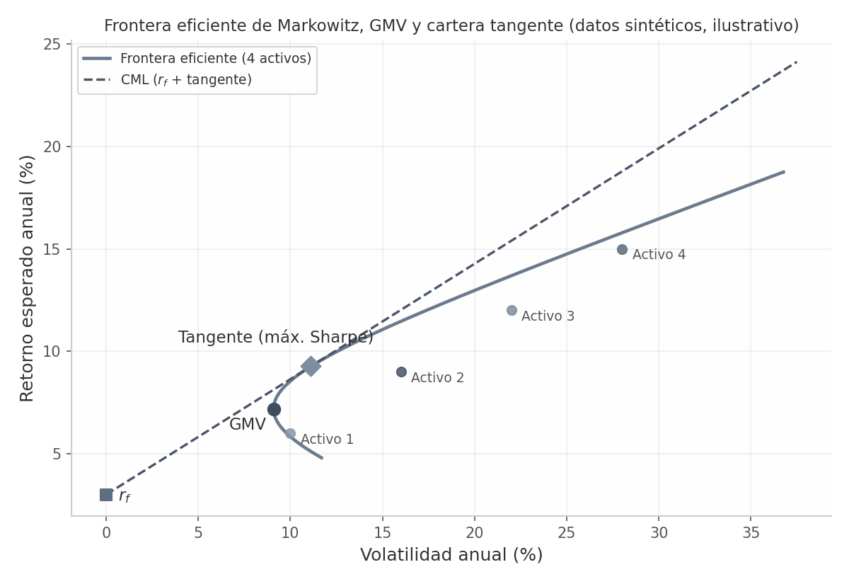
Figure 8.1. Markowitz efficient frontier with four synthetic assets: global minimum-variance portfolio (GMV) and tangency portfolio on the Capital Market Line. Own elaboration with synthetic data, Jul 2026.
Tobin's two-fund separation. Tobin (1958) showed that the choice of which risky portfolio to hold is independent of risk aversion: only how much is invested in it versus the safe asset changes (arXiv.org) . Every optimal portfolio is:
with \(y > 1\) implying leverage. The conservative and the aggressive investor hold the same risky portfolio; they differ only in the leverage applied to it (稀土掘金) .
CAPM. In equilibrium, the tangency portfolio is the market portfolio and every asset prices on the Security Market Line (Sharpe 1964; Lintner 1965; Mossin 1966) (mer.vin) :
Factor models. The single-factor CAPM generalizes into the factor decomposition of returns. Fama-French 3 factors (1993) adds size and value, explaining roughly 90% of the variation of diversified portfolios versus the CAPM's ~70% (Github) :
Carhart (1997) adds momentum \(WML\) (Winners Minus Losers, winners 12–1 months minus losers) (Github) :
and Fama-French 5 factors (2015) incorporates operating profitability (\(RMW\), Robust Minus Weak) and conservative investment (\(CMA\), Conservative Minus Aggressive) (Github) :
These models matter here for two reasons: (i) they define the factor risk budgets that are imposed as linear constraints in the optimizer (\(\sum_i w_i \beta_{i,k} \leq b_k\)), and (ii) they are the benchmark that any "alpha" generated by an LLM must beat net of costs —section 8.4 will show that LLM styles are usually undeclared FF/Carhart factor exposures (Github) . Factor data are downloaded from the Ken French Data Library (Github) .
In plain terms: the efficient frontier is the menu of undominated routes
Think of planning a road trip. Some routes are dominated: there is another one that gets you there just as fast with less dangerous stretch, or sooner with the same risk. Nobody would choose those. The efficient frontier is, simply, the set of routes that are not dominated: each point offers the maximum possible return for its level of risk. On that menu there are two stops with their own names:
- The GMV (global minimum variance) is the calmest route of all, no matter what time you arrive. Since it does not use expected returns —only the covariance matrix—, it is the most robust option of the family: it spares itself the noisiest datum of the problem, as section 8.2 will quantify.
- The tangency portfolio is the route with the best "progress per unit of fright": it maximizes the excess return over \(r_f\) per point of volatility. Tobin showed that all investors should travel the same risky stretch (the tangency) and differ only in how much of the trip they make on it versus the safe highway of the risk-free asset.
The price of that elegance: the tangency portfolio depends entirely on \(\boldsymbol{\mu}\) and on inverting \(\boldsymbol{\Sigma}\). That is where all the problems of the module begin.
8.1.2 Black-Litterman, Kelly and the \(\boldsymbol{\mu}\)-free methods
Full Black-Litterman. Black and Litterman (1992) solved the absurd-inputs problem of MVO by reversing the direction of the calculation: instead of estimating \(\boldsymbol{\mu}\) and optimizing, they start from CAPM equilibrium and let the investor tilt the prior only where they have conviction (Github) . The procedure has four steps.
Step 1 — Implied equilibrium returns (reverse optimization on the market-cap weights \(\mathbf{w}_m\), with \(\delta\) typically between 2.5 and 3.5) (Github) :
Step 2 — Investor views: \(k\) views \(\mathbf{q} = P\boldsymbol{\mu} + \boldsymbol{\varepsilon}\), with \(\boldsymbol{\varepsilon} \sim \mathcal{N}(\mathbf{0}, \boldsymbol{\Omega})\), \(P \in \mathbb{R}^{k \times n}\) "picking" matrix and \(\boldsymbol{\Omega}\) the uncertainty diagonal.
Step 3 — Bayesian posterior, in its two equivalent exact forms (Github) :
with posterior covariance \(\boldsymbol{\Sigma}_{BL} = \boldsymbol{\Sigma} + M\), where \(M = \left[(\tau\boldsymbol{\Sigma})^{-1} + P^\top \boldsymbol{\Omega}^{-1} P\right]^{-1}\). The scalar \(\tau\) measures the uncertainty of the prior; institutional practice sets it in \([0{,}01, 0{,}05]\) or as \(\tau = 1/T\) (Github) . Idzorek's (2005) calibration of \(\boldsymbol{\Omega}\) sets each diagonal element from the variance of the view's asset combination (Github) :
Step 4 — Weights: \(\boldsymbol{\mu}_{BL}\) and \(\boldsymbol{\Sigma}_{BL}\) are fed to the MV optimizer: \(\mathbf{w}^* = \frac{1}{\delta}\boldsymbol{\Sigma}_{BL}^{-1}\boldsymbol{\mu}_{BL}\) (unconstrained). The economic reading is the pedagogical key: BL is a Bayesian shrinkage toward equilibrium —a view with high \(\Omega\) barely moves \(\boldsymbol{\pi}\); a view with low \(\Omega\) dominates it locally. That is exactly where the LLM views of section 8.3 will enter.
Kelly criterion. Kelly (1956) maximizes the expected logarithmic growth rate of wealth (Github) . For a bet with probability \(p\) of winning and net odds \(b\):
Differentiating and setting to zero yields the optimal fraction (Github) :
The generalization with partial losses (Rotando and Thorp 1992; Thorp 2008), where \(a\) are the odds of the negative outcome (Github) :
and the Gaussian continuous version, with its multivariate form (Github) :
Multivariate Kelly coincides with the unnormalized tangency portfolio —the \(\lambda = 1\) case of MVO—, which connects sizing and optimization in a single theory. Since full Kelly is extraordinarily sensitive to the estimated edge, standard practice is fractional Kelly \(\hat{f} = c \cdot f^{*}\) with \(c = 1/2\) or \(1/4\): half-Kelly retains roughly 75% of the growth with about half the volatility, and Thorp himself operated in that range (Github) .
Equal Risk Contribution (ERC). Risk-only methods remove \(\boldsymbol{\mu}\) from the problem. The marginal risk contribution and the risk contribution of asset \(i\) are (Maillard, Roncalli and Teïletche 2010) (Github) :
By the Euler identity of Module 7, \(\sigma_p = \sum_i RC_i\). The ERC condition requires each asset to contribute exactly \(1/n\) of total risk:
With no general closed-form solution, it is solved numerically (least-squares formulation; Spinu's 2013 version convexifies the problem via a logarithmic function) (Github) :
ERC sits between \(1/N\) and GMV on the diversification-risk spectrum.
Ledoit-Wolf covariance shrinkage. The sample covariance \(S\) is noisy and ill-conditioned; the Ledoit-Wolf estimator (2003/2004) combines it convexly with a structured target \(F\) (Source) :
with optimal intensity computable in closed form from the data, with no free parameters (AgentConn) :
Usual targets: constant correlation (2003: \(f_{ii} = s_{ii}\), \(f_{ij} = \bar{\rho}\sqrt{s_{ii}s_{jj}}\)) and scaled identity (2004: \(F = \frac{\operatorname{Tr}(S)}{n} I\)). Verified numerical example: with \(\delta = 0{,}45\), sample correlation 0.72 and mean 0.42, the shrunk correlation is \(0{,}45 \times 0{,}42 + 0{,}55 \times 0{,}72 = 0{,}585\) (maryammiradi.com) . Course operating rule: never feed raw sample \(\Sigma\) to BL or MVO with more than a dozen assets.
Maximum Diversification. Choueifaty and Coignard (2008) maximize the diversification ratio (TradingAgents-AI) :
The solution without the no-shorting constraint is \(\mathbf{w}_{MD} \propto \boldsymbol{\Sigma}^{-1} \boldsymbol{\sigma}\), normalized to sum 1 (Cambridge University Press & Assessment) . If all Sharpes are equal, MDP coincides with the tangency portfolio; moreover, \(DR^2\) is the effective number of independent risk sources in the portfolio (Cambridge University Press & Assessment) .
HRP — Hierarchical Risk Parity. López de Prado (2016) achieves diversification without inverting \(\boldsymbol{\Sigma}\), eliminating at the root the instability of \(\boldsymbol{\Sigma}^{-1}\) (ResearchGate) . Three stages: (1) hierarchical clustering on the correlation-derived distance:
(2) quasi-diagonalization: reordering the rows and columns of \(\boldsymbol{\Sigma}\) following the dendrogram so that similar assets end up adjacent; (3) recursive bisection: for each split into subclusters \(c_1, c_2\), the intra-cluster variance is computed with inverse-variance allocation,
and the split factor between subclusters:
Weights propagate multiplicatively down to the leaves. Documented extensions include HERC/HERC2 (Raffinot 2018), NCO (López de Prado 2019) and Schur complementary allocation (Cotton 2024), which unifies HRP and minimum variance while guaranteeing \(\text{var}(\text{Schur}) \leq \text{var}(\text{HRP})\) (arXiv.org) .
HRP and fractional Kelly in production:
from pypfopt import HRPOpt

hrp = HRPOpt(returns)                 # Ward clustering + recursive bisection
w_hrp = hrp.optimize()                # without inverting Sigma: robust to ill-conditioning

# Fractional Kelly on the BL tangency portfolio (prudential sizing)
f_kelly_full = np.linalg.solve(S_bl.values, mu_bl.values - 0.03)   # Sigma^-1 (mu - rf 1)
c_frac = 0.25                                                         # quarter-Kelly
w_final  = c_frac * f_kelly_full / np.sum(np.abs(f_kelly_full))
Reference implementation (PyPortfolioOpt):
from pypfopt import EfficientFrontier, risk_models, expected_returns

mu = expected_returns.mean_historical_return(prices)
S  = risk_models.CovarianceShrinkage(prices).ledoit_wolf()   # never raw sample_cov
ef = EfficientFrontier(mu, S)
w_tan = ef.max_sharpe(risk_free_rate=0.03)

ef_gmv = EfficientFrontier(mu, S)
w_gmv  = ef_gmv.min_volatility()
GMV with cvxpy (full constraint control):
import cvxpy as cp
import numpy as np

n = S.shape[0]
w = cp.Variable(n)
prob = cp.Problem(
    cp.Minimize(cp.quad_form(w, S.values)),
    [cp.sum(w) == 1, w >= 0, w <= 0.25]        # long-only + per-asset cap
)
prob.solve()
w_gmv = w.value                                 # constrained GMV = implicit shrinkage (§8.2)
Worked example: full, half and quarter Kelly, number by number
A strategy wins with probability \(p = 0{,}60\) and pays net odds \(b = 1\) (it wins exactly what was bet). The module's discrete formula, \(f^{*} = p - (1-p)/b\), gives \(f^{*} = 0{,}20\): full Kelly would bet 20% of capital on each occasion. How much growth is sacrificed by fractioning? Evaluating the logarithmic growth rate \(G(f) = p\ln(1+bf) + (1-p)\ln(1-f)\):
import numpy as np

def G(f, p=0.60, b=1.0):
    return p * np.log(1 + b * f) + (1 - p) * np.log(1 - f)

f_star = 0.60 - 0.40 / 1.0                          # 0.20
for c in (1, 1/2, 1/4):
    f = c * f_star
    print(f"c={c:<5} f={f:.3f}   G={G(f):.4%}   retencion={G(f)/G(f_star):.1%}")
# c=1     f=0.200   G=2.0136%   retencion=100.0%
# c=0.5   f=0.100   G=1.5042%   retencion=74.7%
# c=0.25  f=0.050   G=0.8757%   retencion=43.5%
Three readings. First, the table confirms the module's figure: half-Kelly retains ~75% of expected growth in exchange for roughly half the trajectory volatility (exercise 3 simulates it with 1,000 trajectories). Second, quarter-Kelly —the \(c = 0{,}25\) of the HRP/Kelly snippet in this very section— retains only 43%: it is insurance against overestimating the edge, not a maximization. If the real \(p\) were 0.55 instead of 0.60, true Kelly would be 0.10 and betting 20% would be over-leverage. Third, the connection with Markowitz: multivariate Kelly \(\mathbf{f}^{*} = \boldsymbol{\Sigma}^{-1}(\boldsymbol{\mu} - r_f\mathbf{1})\) is the unnormalized tangency portfolio, so all the fragility of section 8.2 applies to sizing as well —fractioning \(f\) is the sizing equivalent of shrinkage in allocation.
8.2 The fragility of optimization
8.2.1 Error maximization, estimation sensitivity and defenses
The enemy is the input, not the model. Merton (1980) showed that the covariance matrix can be estimated with high precision using data of reasonable frequency, but that the mean of returns is only estimable with histories far longer than those available: with realistic historical data, \(\hat{\boldsymbol{\mu}}\) is essentially useless for computing optimal weights (B2BITS) . Chopra and Ziemba (1993) quantified the damage hierarchy: errors in means have roughly an order of magnitude more impact on utility loss than errors in variances, and these in turn more than errors in covariances —the commonly cited rule of thumb is ~11× means versus variances and ~21× means versus covariances in certainty-equivalent terms, figures best taken as an order of magnitude and not as a universal constant. The didactic consequence is direct: the research budget should go first to \(\boldsymbol{\mu}\), not to \(\boldsymbol{\Sigma}\).
The geometric mechanism is the inversion of \(\boldsymbol{\Sigma}\): in correlated universes the matrix is nearly singular and multiplying by \(\boldsymbol{\Sigma}^{-1}\) amounts to multiplying by a large number, which magnifies small changes in expected returns into huge changes in weights (Best and Grauer 1991). The canonical numerical example: with correlation 0.7, changing one asset's expected return by only 2 percentage points (from 10% to 8%) reduces its optimal weight from 0.50 to 0.18 (B2BITS) . The following figure reproduces the phenomenon with the four synthetic assets: moving Asset 4's expected return by \(\pm 2\) pp. shifts its tangency weight from 12.2% to 26.1% —almost 14 pp. of rotation from a perfectly plausible estimation error.
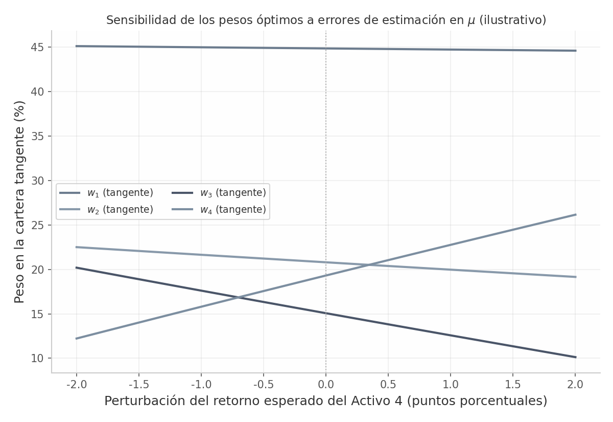
Figure 8.2. Sensitivity of tangency-portfolio weights to a ±2 pp. perturbation in Asset 4's expected return: its weight moves from 12.2% to 26.1%. Own elaboration with synthetic data, Jul 2026.
Michaud and the \(1/N\) verdict. Michaud (1989) named the phenomenon: MVO is an error maximization device that aggressively exploits estimation errors instead of approximating the true mean-variance trade-off (Github) . The formal line starts with Jobson and Korkie (1980), continues with Britten-Jones (1999) —the sampling error of tangency weights is enormous— and with Green and Hollifield (1992), who show that even without estimation error a dominant factor generates extreme weights (Foxholm Financial) . The most uncomfortable empirical result is DeMiguel, Garlappi and Uppal (2009): fourteen sophisticated strategies (Bayes-Stein, minimum variance, constraints) against \(1/N\) on seven datasets, and none consistently beats the equal-weight allocation out of sample; with costs, the gap widens (Github) . The caveat documented by Kirby and Ostdiek (2012) is equally important: much of the result comes from a design with high estimation risk and extreme turnover, and low-turnover MVO (volatility/reward-to-risk timing) can indeed beat \(1/N\) net of costs (Github) .
Constraints as shrinkage (Jagannathan-Ma). The most counterintuitive and most useful result in the literature: the long-only GMV portfolio with upper caps computed with \(\hat{\boldsymbol{\Sigma}}\) is identical to the unconstrained GMV of a modified matrix in which the Lagrange multipliers shrink the covariances of the assets at the cap. Imposing "wrong" constraints acts as covariance shrinkage, and that is why the constrained GMV beats the unconstrained one out of sample (Jagannathan and Ma 2003) (arXiv.org) . DeMiguel, Garlappi, Nogales and Uppal (2009) unified the landscape: norm constraints \(\|\mathbf{w}\|_p \leq \delta\) nest as special cases Ledoit-Wolf shrinkage, the Jagannathan-Ma result and \(1/N\) itself (tessl.io) . Operational lesson: sector constraints, per-asset caps and long-only are not concessions to compliance; they are statistical regularization.
Turnover and costs. Net return after rebalancing incorporates the transaction cost \(\phi\) (Palomar 2025) (arXiv.org) :
with a linear model \(\phi = \sum_i c_i |w_i^{reb} - w_i^{drift}|\) for commissions and spread, and market impact quadratic in weights (square root in volume, Almgren-Chriss; Module 7). The standard defense is to penalize turnover inside the objective (arXiv.org) :
For illustration: 200% annual turnover on a 100-million portfolio with an average effective cost of 15 bps per side destroys 300,000.00 of annual return (30 bps of drag) —enough to reverse the ranking of any pair of methods in the table below.
Deflated Sharpe Ratio. Every allocation backtest must be corrected for sample length, non-normality and selection bias from multiple trials (Bailey and López de Prado 2014) (Github) :
where \(E[\max SR]\) is the maximum expected Sharpe under the null after \(N\) independent trials:
with \(\zeta\) the Euler-Mascheroni constant and \(V_{SR}\) the variance of the Sharpes across trials. Practical rule: require \(DSR > 0{,}95\), complemented with PBO via CSCV and purged/embargoed cross-validation for series with overlapping labels (Github) .
Table 8.1 — Allocation methods: assumptions, critical inputs, fragility and when to use them
| Method | Key assumptions | Critical inputs | Dominant fragility | When to use it |
|---|---|---|---|---|
| GMV | Only risk matters; \(\boldsymbol{\mu}\) ignored | \(\boldsymbol{\Sigma}\) (well estimated) | Estimation of \(\boldsymbol{\Sigma}\); concentration in low-vol assets | Robust baseline; broad universe with little return signal |
| Tangency (max Sharpe) | \(\boldsymbol{\mu}\), \(\boldsymbol{\Sigma}\) known; \(r_f\) exists | \(\boldsymbol{\mu}\) and \(\boldsymbol{\Sigma}^{-1}\) | Extreme error maximization: \(\pm 2\) pp. in \(\mu_i\) → ±14 pp. in \(w_i\) | Only with shrunk \(\boldsymbol{\mu}\) (BL, Bayes-Stein) and constraints |
| Black-Litterman | CAPM equilibrium as prior; views \(\sim \mathcal{N}\) | \(\mathbf{w}_m\), \(\delta\), \(\tau\), \(P\), \(\mathbf{q}\), \(\boldsymbol{\Omega}\) | Poor calibration of \(\boldsymbol{\Omega}\); overconfident views | Whenever there are views (human or LLM) to combine with the market |
| Kelly (fractional) | Estimable edge; logarithmic utility | Edge (\(p\), \(b\) or \(\mu/\sigma^2\)) | Overestimating the edge → ruinous over-leverage | Sizing bets with documented edge; always \(c \leq 1/2\) |
| ERC / Risk Parity | Diversification by risk, not capital | \(\boldsymbol{\Sigma}\) | Rotation toward low-vol/estimated-correlation assets | Multi-asset portfolios without reliable return views |
| Maximum Diversification | Maximize \(DR\); implicit homogeneous Sharpes | \(\boldsymbol{\Sigma}\), \(\boldsymbol{\sigma}\) | \(\boldsymbol{\Sigma}^{-1}\) reappears; sensitive to conditioning | When equal ex-ante Sharpes are believed and maximum diversification is wanted |
| HRP | Hierarchical correlation structure | \(\boldsymbol{\Sigma}\) (not inverted), linkage | Arbitrariness of clustering; less efficient in-sample | Production with ill-conditioned \(\boldsymbol{\Sigma}\) or large \(n\) |
Interpretation. The table orders the methods from highest to lowest dependence on \(\boldsymbol{\mu}\), which is exactly the order from highest to lowest fragility: the tangency portfolio concentrates all the theory and all the estimation risk; GMV, ERC, MDP and HRP deliberately give up the noisiest input in exchange for less ambitious objectives. Black-Litterman sits in the middle because it does not eliminate \(\boldsymbol{\mu}\) but anchors it: the equilibrium prior acts as structural shrinkage and views only shift the posterior where \(\boldsymbol{\Omega}\) allows. Kelly is not a rival allocation method but a sizing rule that, in its multivariate form, coincides with the unnormalized tangency portfolio —its fragility is therefore the same, amplified by leverage. The "when to use it" column summarizes the course doctrine: the method is chosen according to the quality of the available information, not its mathematical sophistication; with weak, noisy views (including an LLM's), BL with high \(\boldsymbol{\Omega}\) or \(\boldsymbol{\mu}\)-free methods dominate the naive tangency portfolio.
Common pitfall: feeding raw \(\hat{\boldsymbol{\mu}}\) to max_sharpe
The reference snippet of section 8.1.2 teaches the PyPortfolioOpt API: mean_historical_return + ledoit_wolf + max_sharpe. The production mistake is reading it as a recipe: that sequence feeds the optimizer the sample historical mean, precisely the input Merton (1980) declared essentially inestimable with the available histories, and whose errors weigh on the order of 11× more than those of variances and 21× more than those of covariances (Chopra-Ziemba). The module's own Figure 8.2 quantifies it: ±2 pp. in one asset's expected return moves its tangency weight from 12.2% to 26.1%.
The snippet teaches syntax; Table 8.1 teaches doctrine: the tangency portfolio only enters production "with shrunk \(\boldsymbol{\mu}\) (BL, Bayes-Stein) and constraints". Operational translation with the defenses already seen in the module:
- Anchor the return: use the Black-Litterman posterior \(\boldsymbol{\mu}_{BL}\) or shrink \(\hat{\boldsymbol{\mu}}\) toward \(\mu_{\text{GMV}}\) (exercise 5), never the raw mean.
- Constrain on purpose: long-only and per-asset caps are not compliance; they are covariance shrinkage via Jagannathan-Ma.
- Charge for changing your mind: penalize turnover in the objective, because 30 bps of annual drag are enough to reverse the ranking between methods.
If your pipeline includes none of the three, you do not have a tangency portfolio: you have noise amplified by \(\boldsymbol{\Sigma}^{-1}\).
Choosing the method according to the available information (and the toll of rebalancing)
The interpretation of Table 8.1 summarizes the course doctrine: the method is chosen by the quality of the available information, not by its mathematical sophistication. This map turns it into a procedure:

And one toll the map does not draw but the committee does pay: changing allocation costs money. With the module's linear model, \(\phi = \sum_i c_i|w_i^{reb} - w_i^{drift}|\), the annual drag is proportional to turnover:
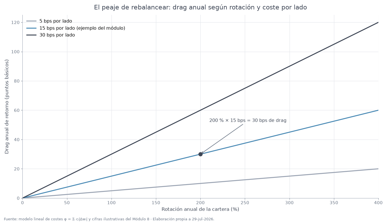
Figure E8.1. Annual drag in basis points for effective costs of 5, 15 and 30 bps per side. The marked point reproduces the module's numerical example: 200% turnover × 15 bps = 30 bps of drag, i.e., USD 300,000 per year on a USD 100 M portfolio —enough to reverse the ranking of Table 8.1. Source: illustrative figures from the module · Own elaboration as of 29-Jul-2026.
That is why the operative version of the objective penalizes \(\gamma\sum_i|w_i - w_i^{prev}|\): it is not decorative prudence, it is what separates a winning backtest from a real portfolio with positive net return.
8.3 LLM views for Black-Litterman (full practical case)
8.3.1 Documented pipeline: from news to weights with human veto
The best empirically supported integration is Kim, Lee et al. (2025, arXiv 2504.14345), a complete and reproducible framework: for each stock in the universe (S&P 500) the LLM is queried \(N = 100\) times with recent news; the mean of the repeated responses constitutes the views vector \(\mathbf{q}\), and the variance of the responses populates the diagonal of \(\boldsymbol{\Omega}\) —higher variance implies higher uncertainty and, automatically, lower weight of the view in the posterior—, with \(P = I\) (one absolute view per asset) (tessl.io) . The reported result is that portfolios guided by the best-performing LLMs outperform traditional baselines in absolute and risk-adjusted terms, but —an essential caveat— the choice of LLM is not the search for a better forecaster but "a strategic choice of investment style whose success depends on its alignment with the prevailing market regime" (tessl.io) . The equivalent GLS specification used by the paper makes the stacked prior-and-views structure explicit (Cambridge University Press & Assessment) :
The full institutional pipeline, with LangChain/LangGraph at the view-generation layer and deterministic tools downstream, respects the course's backbone pattern: the LLM reasons, the math decides, the human vetoes.

Snippet — view-generation layer with LangChain (structured output, closed schema):
from pydantic import BaseModel, Field
from langchain_openai import ChatOpenAI

class VistaActivo(BaseModel):
    ticker: str
    retorno_esperado_anual: float = Field(description="Vista de retorno, en tanto por uno")
    justificacion: str = Field(max_length=500)
    evidencia_literal: str = Field(description="Cita verbatim de la noticia que sustenta la vista")

llm = ChatOpenAI(model="gpt-5", temperature=1.0)   # temperature > 0: dispersion is the signal
chain = llm.with_structured_output(VistaActivo)

# N = 100 repeated queries per asset (arXiv 2504.14345)
respuestas = [chain.invoke({"noticias": noticias_pit, "ticker": tk}) for _ in range(100)]
q_i     = float(np.mean([r.retorno_esperado_anual for r in respuestas]))
omega_i = float(np.var([r.retorno_esperado_anual for r in respuestas], ddof=1))
Two design decisions are non-negotiable. First, the closed schema with literal evidence: each view must quote verbatim the news item that supports it (the anti-hallucination discipline of Module 6), and the news must be point-in-time —published before the decision timestamp, with ingestion latency modeled—. Second, temperature is not minimized: the dispersion of the responses is the measure of uncertainty that feeds \(\boldsymbol{\Omega}\).
Snippet — BL posterior with PyPortfolioOpt and constrained optimization:
from pypfopt.black_litterman import BlackLittermanModel

bl = BlackLittermanModel(
    S_lw,                                # Ledoit-Wolf covariance (never raw sample)
    pi="market_cap",                     # equilibrium prior: pi = delta Sigma w_m
    absolute_views=pd.Series(q_dict),    # q: means of the N=100 queries
    omega="idzorek",                     # or diagonal = variance of the queries
    tau=0.025,
)
mu_bl   = bl.bl_returns()
S_bl    = bl.bl_cov()
ef      = EfficientFrontier(mu_bl, S_bl)
ef.add_constraint(lambda w: w >= 0)                  # long-only
ef.add_constraint(lambda w: w <= 0.10)               # per-asset cap (Jagannathan-Ma)
weights = ef.max_sharpe(risk_free_rate=0.03)         # -> human veto before the OMS
In institutional practice. The documented deployment closest to this pipeline in production combines three conservative decisions. (i) Small, liquid universe: views are issued on mega-caps where the error of \(\hat{\boldsymbol{\mu}}\) is least damaging and borrow is not a problem. (ii) Deliberately inflated \(\boldsymbol{\Omega}\): the variance of the \(N\) queries is multiplied by a prudential factor (typically 2–5) before entering BL, because the evidence of section 8.4 shows that the LLM's linguistic confidence is not a tradable probability (Github) . (iii) Human veto with a trail: the committee logs each approval/veto together with the views JSON, the prompt version and the LangSmith trace, so the decision is reconstructible before an auditor —the same observability discipline that the governance module requires as the only defense against the regulatory vacuum of agentic AI. The arXiv 2504.14345 pipeline is used as a reproducible academic reference, not as a deployment template: its results are an object of study (short windows, incomplete frictions), not a strategy.
Critical context of the case. The headline-sentiment signal has the best empirical pedigree in the LLM literature (Lopez-Lira and Tang 2023: post-cutoff GPT-4 scores that predict the initial reaction and the subsequent drift, stronger in small-caps and negative news), but the authors themselves document that "strategy returns decay as LLM adoption increases, consistent with improved price efficiency" —the edge gets arbitraged away (skfolio.org) . And Glasserman and Lin (2023) decompose the bias into look-ahead and distraction effect: in-sample, anonymized headlines perform better than identified ones, because general knowledge of the company contaminates the sentiment reading more than recall of the future —especially in large caps—, which turns headline anonymization into standard de-biasing procedure before generating views (Cambridge University Press & Assessment) .
Worked example: from repeated responses to a view \((q_i, \omega_i)\)
Suppose that for the asset ACME the module's pipeline returns these five readings of retorno_esperado_anual (in production there are \(N = 100\) queries; we use five so the calculation can be verified by hand): [0.14, 0.10, 0.17, 0.11, 0.13].
Step by step:
- The view is the mean: \(q_i = (0{,}14 + 0{,}10 + 0{,}17 + 0{,}11 + 0{,}13)/5 = 0{,}13\), a 13% expected return.
- The uncertainty is the sample variance (
ddof=1): the deviations are \(0{,}01,\ -0{,}03,\ 0{,}04,\ -0{,}02,\ 0{,}00\); their squares sum \(0{,}0001 + 0{,}0009 + 0{,}0016 + 0{,}0004 + 0 = 0{,}0030\), and \(\omega_i = 0{,}0030/4 = 0{,}00075\) (a typical dispersion of ~2.7 pp.). - The prudential factor: section 8.4 shows that linguistic confidence is not a tradable probability, so institutional practice multiplies \(\omega_i\) by 2–5. With 3: \(\omega_i^{prud} = 0{,}00225\).
muestra = [0.14, 0.10, 0.17, 0.11, 0.13]     # illustration; production: N = 100
q_i     = float(np.mean(muestra))            # 0.13
omega_i = float(np.var(muestra, ddof=1))     # 0.00075
omega_prudente = 3.0 * omega_i               # 0.00225

bl = BlackLittermanModel(
    S_lw,                                    # Ledoit-Wolf covariance, as in the module
    pi="market_cap",
    absolute_views=pd.Series({"ACME": q_i}),
    omega=np.diag([omega_prudente]),         # diagonal = variance of the queries
    tau=0.025,
)
The contrast is the lesson. If the five responses had been identical, \(\omega_i \approx 0\) and Black-Litterman would take the view almost as certainty: the posterior would stick to 0.13. With the observed dispersion —inflated by the prudential factor—, \(\boldsymbol{\mu}_{BL}\) barely separates from \(\boldsymbol{\pi}\) for that asset. That is why temperature is not minimized: dispersion is the thermometer, and an LLM that "hesitates" produces views the model itself automatically downgrades. And mind the nuance: the decoder always answering the same does not prove certainty, it proves decoder determinism —one more reason to inflate \(\boldsymbol{\Omega}\).
8.4 Critical evidence on LLMs and prediction
8.4.1 Memorization, Alpha Illusion and the consequence for \(\boldsymbol{\Omega}\)
Four results delimit what an LLM can contribute to portfolio construction.
Memorization Problem. Lopez-Lira, Tang and Zhu (2025) —the same first author of the foundational pro-predictability paper, in a remarkable self-correction by the community— show that LLMs recall with recall-precision the exact values of economic variables prior to their cutoff (MAE of 0.03%–0.15% on unemployment, GDP and S&P 500; directional accuracy above 96%), that neither explicit instructions to respect temporal boundaries nor masking prevents it, and that post-cutoff the recall disappears (arXiv.org) . Devastating conclusion: one cannot tell whether the LLM is forecasting or accessing memorized data; every backtest of LLM views inside the training window is contaminated.
Alpha Illusion and reproducibility. "The Alpha Illusion" audit (2026) of FinCon, FinMem, TradingAgents, FinAgent, QuantAgent and FLAG-Trader concludes that the alpha reported by end-to-end LLM agents should not be treated as deployment evidence: current public evidence does not distinguish robust predictive ability from temporal contamination, unmodeled frictions, Sharpe uncertainty in short windows, narrative fitting and parametric priors (Github) . The "Agentic Trading" audit (2026) protocolizes 77 empirical studies and reports that zero meet the full reproducibility criteria (arXiv.org) ; "Profit Mirage" (2025) quantifies how dazzling returns evaporate once the model's knowledge window ends (arXiv.org) . Look-ahead is structural in pre-trained language models (Sarkar and Vafa 2024) (Github) .
Why LLMs do not beat systematic factors. The few works with rigorous factor control show that sentiment "alpha" shrinks substantially after adjusting for Fama-French and costs; the documented survival corresponds to small specialized models trained year by year (FinText, by Rahimikia and Drinkall), not to generalist LLMs (metricgate.com) . Moreover, the "styles" LLMs exhibit in the enhanced BL are undeclared implicit factor exposures: when the model "chooses" small-caps or value, it is replicating known FF/Carhart premia without attribution (Github) . The honest comparison standard remains Gu, Kelly and Xiu (2020).
Operational implication for the section 8.3 pipeline. LLM views are treated as a weak signal with high \(\boldsymbol{\Omega}\), never as truth: (i) evaluate only post-cutoff or with living benchmarks; (ii) anonymize headlines (anti-distraction); (iii) inflate \(\boldsymbol{\Omega}\) with a prudential factor; (iv) validate the full system with DSR > 0.95 and PBO; (v) attribute the result against FF5/Carhart factors before claiming alpha.
Table 8.2 — Critical evidence on LLMs in financial prediction
| Paper | Finding | Documented bias |
|---|---|---|
| Lopez-Lira & Tang (2023, arXiv 2304.07619) | Post-cutoff GPT-4 scores predict initial reaction (~90% hit rate portfolio-day, not tradable) and drift; long-short Sharpe 3.8 (v4) → 3.28 (v5) | No costs; numbers change across versions; decay with adoption |
| Glasserman & Lin (2023, arXiv 2309.17322) | Anonymized headlines perform better in-sample: distraction dominates look-ahead | Distraction effect, mostly in large caps |
| Kim, Lee et al. (2025, arXiv 2504.14345) | LLM views (mean of 100 queries, variance → \(\boldsymbol{\Omega}\)) beat baselines; each LLM is a regime-dependent "style" | Styles = implicit factor exposures; short window |
| Lopez-Lira, Tang & Zhu (2025, arXiv 2504.14765) | Exact pre-cutoff recall (>96% directional accuracy; MAE 0.03–0.15%); zero recall post-cutoff | Memorization: forecasting indistinguishable from recall |
| The Alpha Illusion (2026, arXiv 2605.16895) | End-to-end agents' alpha is not deployment evidence; "linguistic confidence is not a tradable probability" | Temporal contamination, omitted frictions, short-window Sharpe |
| Agentic Trading (2026) / Profit Mirage (2025, arXiv 2510.07920) | 0 of 77 studies fully reproducible; returns evaporate after the cutoff | Parametric leakage; systemic irreproducibility |
Interpretation. The table does not contradict section 8.3: it bounds it. The first row shows that the sentiment signal is real in the narrow econometric sense —post-cutoff score-return correlation—, but its quantitative headline is unstable (the Sharpe itself is revised downward between paper versions) and gets arbitraged with adoption. Rows two and three explain how to extract that signal without self-deception: anonymize to neutralize distraction, and use the dispersion of repeated queries as an honest measure of uncertainty. The last three rows are the institutional firewall: if the LLM may be recalling rather than reasoning, if 96% pre-cutoff accuracy is memorization, and if no end-to-end study survives a full reproducibility audit, then no LLM view deserves a small \(\boldsymbol{\Omega}\). The resulting architecture —LLM as an auditable information interface upstream, deterministic BL/ERC/HRP engine downstream, human with veto and trail— is not timidity: it is the only position simultaneously compatible with the empirical evidence and with non-delegable regulatory responsibility.
In plain terms: \(\boldsymbol{\Omega}\) is the witness's volume knob
Black-Litterman is, at bottom, a trial with two testimonies: the market's (the equilibrium prior \(\boldsymbol{\pi}\), which summarizes where the billions are placed) and the analyst's (the view \(\mathbf{q}\)). The posterior \(\boldsymbol{\mu}_{BL}\) does not "believe" either of them: it takes an average weighted by each witness's reliability. \(\boldsymbol{\Omega}\) is the second one's volume knob. With low \(\Omega\), the analyst shouts and the posterior shifts to their position; with high \(\Omega\), they whisper and the posterior barely separates from \(\boldsymbol{\pi}\).
All of section 8.4 is the argument for why the LLM has earned the right to speak, but not to shout: it may be recalling (Memorization Problem), getting distracted by the company name (Glasserman-Lin distraction effect), or exhibiting a "style" that is undeclared FF/Carhart factor premia. The practical consequence —LLM views with high \(\Omega\), further inflated by a prudential factor of 2–5— is not gratuitous distrust: it is the exact mathematical translation of "this signal is real but weak".
Common pitfall: the backtest the LLM had already read
The most expensive mistake of this decade in quant research: evaluating LLM views over any period prior to the model's training cutoff. The Memorization Problem (Table 8.2) documents exact recall of pre-cutoff economic values with directional accuracy above 96% —neither explicit instructions nor masking prevent it—, so a 2022 "backtest" with a model trained through 2024 does not measure prediction: it measures memory formatted as a backtest. And the contamination is undetectable by inspecting the code, because it lives in the model's weights.
The minimum protocol the module sets for an evaluation of LLM views to mean anything:
- Post-cutoff only or with living benchmarks that are regenerated: the test data cannot exist in pre-training.
- Anonymized headlines, with no company name or sector, to neutralize the distraction effect.
- Factor attribution: "alpha" is reported net of FF5/Carhart; if the style was undercover value, say so.
- Full statistical validation: DSR > 0.95 and PBO, because a high Sharpe in a short window is luck's favorite format.
If any of the four is missing, the number is not deployment evidence: it is narrative.
Exercises
-
GMV with cvxpy. With the module's four synthetic assets (\(\boldsymbol{\mu} = (0{,}06, 0{,}09, 0{,}12, 0{,}15)\), correlations given), solve the long-only GMV with a 40% per-asset cap using
cvxpy. Numerically verify the closed-form formula \(\mathbf{w}_{\text{GMV}} = \boldsymbol{\Sigma}^{-1}\mathbf{1}/(\mathbf{1}^\top\boldsymbol{\Sigma}^{-1}\mathbf{1})\) without constraints and compare. Repeat with the Ledoit-Wolf shrunk covariance (\(\delta^* = 0{,}45\)) and quantify the change in \(\sigma_{\text{GMV}}\). -
Black-Litterman with simulated LLM views. Starting from \(\boldsymbol{\pi} = \delta\boldsymbol{\Sigma}\mathbf{w}_m\) with \(\delta = 2{,}5\), simulate two absolute "LLM" views: \(\mathbf{q} = (0{,}18, 0{,}02)\) on assets 3 and 4, with \(\omega_1 = 0{,}001\) (confident view) and \(\omega_2 = 0{,}05\) (weak view). Compute \(\boldsymbol{\mu}_{BL}\) with both posterior forms and check that they coincide to machine precision. Then double both \(\omega\) and explain, using the formulas, why the posterior retracts toward \(\boldsymbol{\pi}\).
-
Fractional Kelly. A strategy has \(p = 0{,}55\), \(b = 1\). (a) Compute \(f^*\) with the discrete formula. (b) Plot \(G(f)\) and mark \(f^*\), half-Kelly and quarter-Kelly. (c) Simulate 1,000 trajectories of 252 bets for \(c \in \{1, 1/2, 1/4\}\) and compare median growth, volatility and maximum drawdown. Why does institutional practice choose \(c \leq 1/2\) even though expected growth is lower?
-
HRP versus GMV. With an 8-asset correlation matrix with two strong clusters (intra-cluster correlation 0.7, inter-cluster 0.1), implement HRP recursive bisection (distance \(\sqrt{(1-\rho)/2}\), Ward linkage) and compare the weights and the simulated out-of-sample variance against GMV with sample covariance. Repeat with 60 observations per asset to exacerbate the ill-conditioning of \(\hat{\boldsymbol{\Sigma}}\) and explain the result.
-
Sensitivity and defenses. Perturb each component of \(\hat{\boldsymbol{\mu}}\) by \(\pm 1\) pp. (16 configurations) and record the variation range of the unconstrained tangency weights. Repeat with (a) long-only constraints + 25% cap and (b) \(\boldsymbol{\mu}\) shrunk 50% toward \(\mu_{\text{GMV}}\). Relate the sensitivity reduction to the Jagannathan-Ma theorem.
-
Critical validation. Take the backtest Sharpe from exercise 4, assume \(T = 36\) months, \(\hat{\gamma}_3 = -0{,}5\), \(\hat{\gamma}_4 = 4\) and \(N = 20\) trials with \(V_{SR} = 0{,}25\), and compute the DSR. Does it pass the 0.95 threshold? List which biases from Table 8.2 could be present if the "views" had been generated by an LLM with a cutoff later than the start of the backtest.
Module 8 of 15 — LangChain for Quantitative Trading. Data and versions verified as of July 2026; prices and market figures subject to change. LangChain 1.3.14 / langchain-core 1.5.2.
Elite resources to go deeper
- Kim, Lee et al. (2025) — arXiv 2504.14345: the section 8.3 pipeline as published; note how the variance of the \(N\) queries populates \(\boldsymbol{\Omega}\) and the idea of each LLM as an "investment style".
- Lopez-Lira & Tang (2023) — arXiv 2304.07619: the foundational LLM-sentiment paper; read it with its own caveat about edge decay with adoption.
- Glasserman & Lin (2023) — arXiv 2309.17322: the look-ahead vs. distraction effect decomposition that turns headline anonymization into standard procedure.
- Lopez-Lira, Tang & Zhu (2025) — arXiv 2504.14765: the Memorization Problem, the firewall for any backtest of LLM-generated views.
- Ledoit & Wolf — "Honey, I Shrunk the Sample Covariance Matrix": the shrinkage the module turns into an operating rule; short, elegant and with closed form for \(\delta^{*}\).
- PyPortfolioOpt — BlackLittermanModel documentation: the exact API the module uses (
pi="market_cap",omega="idzorek", absolute views) with all its options. - Ken French Data Library: the FF3/FF5/Carhart factors for the attribution that section 8.4 requires before claiming alpha.
- LangChain — structured output: official documentation for
with_structured_output, the mechanism behind theVistaActivoschema with literal evidence.
Check your understanding
Self-assessment with instant feedback. No scores are stored: it is just for you.