LLM signals and rigorous backtesting
From text to signal, backtests without look-ahead, realistic costs, and the deflated Sharpe ratio.
Learning objectives
Upon completing this module, the reader will be able to:
- Critically evaluate the self-reported results of LLM trading agents (FinMem, TradingAgents, FinCon, HedgeAgents, among others), identifying the documented biases in each paper and separating architectural value from strategy value.
- Integrate an LLM-generated sentiment signal into a classic quantitative pipeline: cross-sectional z-scores, sector neutralization, temporal decay, and novelty weighting.
- Select the appropriate backtesting framework by phase (vectorbt for discovery, zipline-reloaded for cross-sectional factors, LEAN or nautilus_trader for execution validation) and harden it against look-ahead, survivorship, and data snooping.
- Apply the institutional statistical correction: PSR and the Bailey–López de Prado Deflated Sharpe Ratio, PBO via CSCV, and the Harvey–Liu haircut.
- Model realistic transaction costs (implementation shortfall decomposition, Almgren–Chriss optimal trajectory, square-root impact law, borrow on shorts) and quantify the degradation of a raw signal.
- Design a governed execution architecture: signal → deterministic RiskGateway → HITL approval → broker (Alpaca, ib_async, FIX 4.2) with kill switch, in the spirit of SEC 15c3-5.
Modules 7 and 8 equipped the reader with the risk framework and portfolio construction with Black–Litterman views. This module closes Block III by walking the full path from signal to order: what the LLM trading-agent literature really says, how a natural-language output becomes a defensible quantitative signal, how it is validated to the standards an allocation committee would demand, and how it connects to execution without ceding control to a stochastic system. The guiding principle, already anticipated in earlier modules, remains intact: the LLM reasons, the math decides, the human vetoes; agent papers are treated here as an object of study, not as a deployable strategy (ProfitLogic) .
9.1 The state of the art of trading agents
9.1.1 Verified landscape: architectures, headline numbers, and documented biases
Between 2023 and 2026 the academic literature produced a recognizable genealogy of LLM agents for trading: FinMem (arXiv 2311.13743, AAAI Symposium 2024) introduced memory layered by time horizon —shallow layers (daily news, high decay), intermediate (10-Q), and deep (10-K and reflections, low decay)— with a switchable risk profile, and reported Sharpe > 2.0 and cumulative returns > 0.35 on TSLA and NFLX across five mega-caps in 2021–2022 (pfolio.io) . FinAgent (arXiv 2402.18485, KDD 2024) added multimodality (text, numerical series, K-line charts) and double reflection; its abstract headline —92.27% return— comes from one dataset out of six, the exact pattern of best-result selection (arXiv.org) . TradingAgents (arXiv 2412.20138; repo with more than 65,000 stars) simulates a complete firm —four analysts, bull/bear researchers in debate, trader, risk committee, fund manager— and reports CR 26.62% and Sharpe 8.21 on AAPL over a three-month window in 2024, with maximum drawdowns of 0.91% (🦜️🔗 LangChain) . The authors themselves add an unusually honest self-critical footnote: the Sharpe exceeds their expected empirical range (SR > 3 "excellent") and they attribute it to the absence of corrections in the window; with 11 LLM calls and more than 20 tool calls per prediction, they could only test three months (langchain.js) .
StockAgent (arXiv 2407.18957, ACM TIST) makes the methodological contribution of naming the leakage right in the abstract: it is a simulation with an order book and investor personalities explicitly designed to prevent the model from exploiting prior knowledge of the test period (Springer) . FinRobot (arXiv 2405.14767, AI4Finance) is a four-layer analysis platform with a multi-LLM Smart Scheduler, not a trading system; its value is architectural, and its authors criticize the field's obsession with backtesting over process-oriented approaches (rdrr.io) . FinCon (arXiv 2407.06567, NeurIPS 2024 main track) implements a manager–analyst hierarchy with conceptual verbal reinforcement (CVRF) and risk gating with CVaR, reporting CR 113.84% and Sharpe 3.269 on a TSLA/MSFT/PFE portfolio, and being the only agent with a positive return in the TSLA-2022 stress; it also admits hallucinations in memory management (Github) . MarketSenseAI (arXiv 2401.03737, ESWA) reports beating the S&P 100 by 13 points with returns of up to 40% in 2023 —a year inside GPT-4's knowledge window— and declares a conflict of interest: the authors market the framework as a startup (skfolio.org) . HedgeAgents (arXiv 2502.13165, WWW 2025 Companion) reports 70% annualized and 400% over three years, and in the same abstract admits that conventional LLM agents lose ~−20% in fast drawdowns (arXiv.org) .
Table 9.1 — Published LLM trading agents: architecture, reported result, and documented biases
| Paper (venue) | Core architecture | Reported result | Documented biases and caveats |
|---|---|---|---|
| FinMem (AAAI Symp. 2024) | Layered memory + switchable profile | SR > 2.0, CR > 0.35 (TSLA, NFLX) (pfolio.io) | 5 mega-caps, 2021–22; no costs; risk-switching rule fitted ex post; PC = 0.8213 counterfactual leakage (arXiv.org) |
| FinAgent (KDD 2024) | Multimodal + double reflection | 92.27% return (1 dataset out of 6) (arXiv.org) | Best-result selection in the abstract; pure similarity retrieval |
| TradingAgents (arXiv, >65k★) | Multi-agent bull/bear/risk firm | CR 26.62%, SR 8.21 (AAPL) (🦜️🔗 LangChain) | 3-month window; data inside GPT-4's cutoff; authors: SR "outside empirical range" (langchain.js) |
| StockAgent (ACM TIST) | Anti-leakage order book simulation | N/A (behavioral) (Springer) | Not a strategy; behavior reflects the backbone, not the market |
| FinCon (NeurIPS 2024) | Manager–analyst + CVRF + CVaR | CR 113.84%, SR 3.269 (Github) | Oct-2022→Jun-2023 window; admits memory hallucinations (Github) ; partial costs |
| MarketSenseAI (ESWA 2024) | GPT-4 CoT stock selection | +13% vs S&P 100, up to 40% (skfolio.org) | 2023 test in-cutoff; declared commercial conflict of interest (Advisor Perspectives) |
| HedgeAgents (WWW 2025) | Fund manager + hedge experts | 70% annualized, 400%/3 years (arXiv.org) | No independent replication; the paper itself admits −20% under stress (arXiv.org) |
Interpretation. The table summarizes the module's central thesis: the extraordinary numbers always share the same four weaknesses —short window, no costs, data inside the model's knowledge cutoff, and lack of independent replication— and the enthusiast and skeptic literatures do not contradict each other: they measure different objects. FINSABER re-evaluated these strategies over two decades and more than 100 symbols and found that the reported advantages deteriorate significantly, with perverse pro-cyclical behavior: too conservative in bull markets and too aggressive in bear markets (arXiv.org) . DeepFund, in live post-cutoff evaluation, observed net losses even in flagship models (arXiv.org) . The correct professional reading is not cynicism: these architectures —layered memory, adversarial debate, CVaR risk gating— are valuable design patterns for the research scaffolding. What they do not constitute is evidence of deployable alpha; a positive short backtest is not robust alpha, and a plausible narrative is not an operable probability (ProfitLogic) .
Risk note The profit mirage is the most insidious bias in this literature because it lives not in the pipeline but in the model's weights: re-evaluated only with data after their knowledge cutoff, almost all published LLM agents fall to a random baseline, and the best one loses 50% of its performance (arXiv.org) . The arXiv 2505.07078 review further documents that most studies evaluate less than one year, fewer than ten stocks, with no published code and against naive benchmarks (臺灣博碩士論文知識加值系統) . Parametric look-ahead cannot be ruled out by inspecting the pipeline code (Interactive ML) : the only operational defense is strictly post-cutoff backtesting, live benchmarks (DeepFund, StockBench, FinLake-Bench), and counterfactual input-sensitivity tests (arXiv.org) .
In plain terms: why a Sharpe of 8.21 is not a strategy
Evaluating an LLM agent on 2021–2023 data is like examining a student on problems whose solutions had been published for years in the books they studied from: they are not solving, they are remembering. The profit mirage is exactly that — the look-ahead does not live in the pipeline, which can be impeccable, but in the model's weights. That is why Table 9.1 is read professionally with four questions: does the window cover more than one market regime?, are the results net of costs (spread, impact, borrow)?, is the test strictly after the knowledge cutoff?, is there an independent replication? No paper in the table answers yes to all four, and TradingAgents' own authors admit their Sharpe is outside the expected empirical range.
The conclusion is not cynicism: FinMem's layered memory, TradingAgents' bull/bear debate, or FinCon's CVaR gating are reusable design patterns for the research scaffolding. What they do not constitute is evidence of deployable alpha. Applied in cascade, the four-question filter almost never reaches the last one — section 9.1.1 documents that, re-evaluated post-cutoff, almost all published agents fall to the random baseline, and the best loses 50% of its performance. Only what survives all four earns the next phase: 3 to 6 months of paper trading with a pre-registered parity criterion.
9.2 Sentiment as a quantitative signal
9.2.1 Lopez-Lira & Tang, the PEAD evidence, and the integration pipeline
The LLM signal with the best evidence is not an agent architecture but a headline classifier. Lopez-Lira and Tang (arXiv 2304.07619) scored with ChatGPT every common-stock headline from CRSP between October 2021 and December 2022 —after ChatGPT's cutoff, with explicit contamination control— and built a self-financing long-short strategy: Sharpe 3.8 with GPT-4 in the paper's v4, degraded to 3.28 in v5 (and GPT-3.5 from 3.1 to 1.79), versus negative Sharpes for GPT-1/2 and BERT (arXiv.org) . The cumulative return exceeds 500%, but without transaction costs, and with a revealing asymmetry: the short leg contributes 29 bps/day versus 9 bps/day for the long leg —the signal is above all a bad-news detector, concentrated in small-caps where limits to arbitrage make the correction expensive (arXiv.org) . The fact that the numbers change between versions of the same paper is itself a methodological lesson on the fragility of backtests. The PEAD evidence is complementary and of solid pedigree: contextual features from earnings calls improve the per-trade return of a long-short portfolio by 53–354 bps out-of-sample on a point-in-time S&P 500 universe 2010–2022 (fgv.br) , although honest counterexamples exist where text alone does not beat the baseline (Advisor Perspectives) .
Professional integration treats the LLM score as one more factor, not as an order. The reference pipeline: (1) the LLM emits continuous scores (preferable to discrete labels, because they preserve intensity); (2) temporal aggregation with exponential decay —the documented predictability is 1–5 days— and novelty weighting, discounting duplicate or republished headlines; (3) winsorization and cross-sectional z-score by date; (4) neutralization against sector and risk factors (market, size, momentum), keeping the residual; (5) IC-weighted combination with the existing alpha; (6) execution with modeled ingestion lag, because news timestamps record publication, not availability to the pipeline (horizontrading.io) .
where \(s_{i,t}\) is the aggregated news score of asset \(i\) and \(h\) is the signal's half-life (1–3 days in documented practice). Neutralization is implemented as a daily cross-sectional regression of the z-score on sector dummies and factor exposures, using the residual as the final signal.

# --- LLM sentiment signal pipeline → quantitative factor (pandas) ---
import numpy as np, pandas as pd

def agregar_decay(scores: pd.DataFrame, halflife: float = 2.0) -> pd.DataFrame:
    """scores: DataFrame [dates x tickers] of daily LLM scores (NaN = no news).
    Exponential decay with `halflife`-day half-life; only days with news carry weight."""
    lam = np.log(2) / halflife
    out = scores.copy().astype(float)
    for t in range(1, len(out)):
        out.iloc[t] = out.iloc[t].fillna(0) + np.exp(-lam) * out.iloc[t-1].fillna(0)
    return out

def zscore_cross_sectional(sig: pd.DataFrame, win: float = 0.01) -> pd.DataFrame:
    lo, hi = sig.quantile(win, axis=1), sig.quantile(1 - win, axis=1)
    w = sig.clip(lo, hi, axis=0)                      # winsorized by date
    med = w.median(axis=1)                            # cross-sectional median
    mad = w.sub(med, axis=0).abs().median(axis=1)     # cross-sectional MAD
    return w.sub(med, axis=0).div(1.4826 * mad.replace(0, np.nan), axis=0)

def neutralizar(z: pd.DataFrame, sectores: pd.Series) -> pd.DataFrame:
    """Residual of z on sector dummies, by date (cross-sectional OLS)."""
    D = pd.get_dummies(sectores)
    def resid(fila):
        y = fila.dropna(); Xd = D.loc[y.index]
        beta, *_ = np.linalg.lstsq(Xd.values, y.values, rcond=None)
        return y - Xd.values @ beta
    return z.apply(resid, axis=1)
In institutional practice On the desks that do exploit textual signals, the LLM never touches the portfolio engine directly: it produces a score that enters the factor library as one more column, with its IC decay measured weekly and its weight decided by the existing optimizer. The operational rule that separates research from production is threefold: the signal is built only with news ingested before the decision timestamp (with explicit ingestion lag, not the headline's publication timestamp) (horizontrading.io) ; its evaluation is done post-cutoff of the model or with a certified time-cut backbone (arXiv.org) ; and its cost budget is computed before looking at the gross Sharpe, because a high-turnover daily signal concentrates its alpha exactly where costs are highest: small-caps with wide spreads and expensive borrow (arXiv.org) .
Worked example: four tickers, three days, and a neutralized signal
Let's walk the section's pipeline with small but realistic numbers. A universe of four names —AAA and CCC (technology), BBB and DDD (energy)— and daily LLM scores in [−1, 1] (NaN = no news that day):
| Day | AAA | BBB | CCC | DDD |
|---|---|---|---|---|
| 1 | +0.9 | −0.6 | — | +0.2 |
| 2 | — | −0.3 | +0.8 | — |
| 3 | −0.4 | — | — | +0.5 |
Step 1 — Temporal decay. With half-life \(h=2\) days, the daily factor is \(e^{-\lambda}=2^{-1/2}\approx 0{,}707\): yesterday's news weighs 71%, the day before's 50%. The module's agregar_decay function gives, for day 3:
| AAA | BBB | CCC | DDD | |
|---|---|---|---|---|
| Aggregated score | +0.050 | −0.512 | +0.566 | +0.600 |
Note that DDD reaches 0.600 with no news on day 3: it is \(0{,}5 + 0{,}707 \times 0{,}141\), the decay's memory. That is the point — the documented predictability lasts 1–5 days, not one session.
Step 2 — Cross-sectional z-score. zscore_cross_sectional winsorizes (1%/99%) and normalizes by date with median and MAD, robust to outliers. For day 3 (median 0.308; \(1{,}4826 \times\) MAD \(= 0{,}407\)):
| AAA | BBB | CCC | DDD | |
|---|---|---|---|---|
| z-score | −0.634 | −1.974 | +0.634 | +0.715 |
Step 3 — Sector neutralization. neutralizar subtracts, per date, the sector mean (regression on dummies). The energy mean is −0.629 —dragged down by BBB's bad news— and technology's is 0.000:
| AAA | BBB | CCC | DDD | |
|---|---|---|---|---|
| residual | −0.634 | −1.344 | +0.634 | +1.344 |
The lesson is in DDD: its raw z (0.715) looked barely comparable to CCC's (0.634), but DDD is positive despite a sector with negative sentiment; its idiosyncratic component (1.344) is double CCC's. Without neutralizing you would have split the bet almost evenly; with the residual, the long-short portfolio takes DDD against BBB within the energy sector — an idiosyncratic bet, not a covert bet on oil. The code that reproduces it is exactly the module's:
scores = pd.DataFrame(
    [[ 0.9, -0.6,  np.nan, 0.2],
     [np.nan, -0.3, 0.8,  np.nan],
     [-0.4, np.nan, np.nan, 0.5]],
    index=pd.date_range("2026-07-27", periods=3),
    columns=["AAA", "BBB", "CCC", "DDD"])

s   = agregar_decay(scores, halflife=2.0)          # memory with decay
z   = zscore_cross_sectional(s)                    # robust, by date
res = neutralizar(z, pd.Series({"AAA": "Tech", "CCC": "Tech",
                                "BBB": "Energy", "DDD": "Energy"}))
print(res.iloc[-1].round(3))   # AAA -0.634  BBB -1.344  CCC 0.634  DDD 1.344
9.3 Backtesting to institutional standards
9.3.1 Frameworks 2026, traps, and statistical correction
The first architectural decision is not which library but which family: vectorized engines compute the signal over complete arrays and simulate approximate fills at bar close; event-driven engines process events ordered in time and the strategy reacts —high execution fidelity, lower speed (CSDN博客) . The 2026 decision rule: massive signal discovery in vectorbt/vectorbtpro; microstructure validation and the research→live path in nautilus_trader or QuantConnect LEAN; cross-sectional factors in zipline-reloaded (Pipeline API); weight-based allocation in bt (ar5iv) .
Table 9.2 — Backtesting frameworks 2026: architecture, speed, backtest→live parity, and maintenance
| Framework | Architecture / core | Speed | Multi-asset | Backtest→live parity | Maintenance (2026) |
|---|---|---|---|---|---|
| vectorbt (OSS) / vectorbtpro | Vectorized NumPy/Numba; pro adds Numba loops | Very high–extreme | Yes (columns = assets) | Not native ("execute it elsewhere") (Advisor Perspectives) | Community OSS; pro actively maintained by subscription (from ~USD 25/month) (ar5iv) |
| zipline-reloaded | Event-driven + Pipeline API (Python) | Low-medium | Yes, cross-sectional | No (research only) | Community; "glacial" pace (quant67.com) |
| backtrader | Event-driven loop, pure Python | Low (single-threaded) | Yes | Aging integrations | Legacy: stalled project (ar5iv) |
| QuantConnect LEAN | Event-driven, C# + Python wrapper | High (10 years of equities ≈ 33 s cloud) (MDPI) | Yes: equities, options, futures, FX, crypto | Native: same code, 20+ brokers | Very active (16,000+ stars) (MDPI) |
| nautilus_trader | Event-driven actor/bus, Rust core + PyO3 | Very high | Asset-class agnostic, multi-venue | Native: identical code, only the configuration changes (CSDN博客) | Very active (Nautech Systems) |
| bt | Weights/rebalancing engine (Python) | Medium | Yes (ETF/factor baskets) | No | Mature/stable, low activity (ar5iv) |
Interpretation. The consolidated professional pattern is a two-engine pipeline, not a single bet: massive parameter sweeps and ML research in the vectorized engine (where speed allows exploring thousands of configurations —which, it must be said, aggravates the selection problem we will address with the DSR—) and, only if the signal survives the robustness checks, re-implementation in an event-driven engine with backtest-live parity to validate execution assumptions: fills, latency, T+3 settlement, realistic fees and slippage (ar5iv) . One never deploys from the vectorized engine: its bar-close fills are a discovery approximation, not an execution simulation. The code parity of nautilus_trader and LEAN ("identical strategy code" between backtest, sandbox, and live) (CSDN博客) eliminates the entire class of research→production translation errors that historically contaminated strategy deployment.
The four canonical traps each have their detector. Look-ahead: using information not available at decision time —including the LLM case, where the leak is in the model's weights— (臺灣博碩士論文知識加值系統) . Survivorship: universes without delistings, with estimated annual distortions between 0.1% and 0.9% and pre-inclusion bias when using current index constituents (臺灣博碩士論文知識加值系統) . Data snooping / multiple testing: trying many configurations on the same data and reporting the best; the reported Sharpe is almost never a single hypothesis but the maximum of many noisy estimates (RDocumentation) . Selection/reporting: McLean and Pontiff documented average degradations of −26% out-of-sample and −58% post-publication in published predictors (Github) .
The canonical statistical correction is the Probabilistic Sharpe Ratio, which adjusts the estimated Sharpe for non-normality and sample length with Lo's standard error:
where \(T\) is the number of observations, \(\hat{\gamma}_3\) the sample skewness, \(\hat{\gamma}_4\) the kurtosis (3 = Normal), and \(\Phi\) the Normal CDF. The Deflated Sharpe Ratio replaces the benchmark \(SR^*\) with the expected maximum under the null hypothesis of \(N\) attempted strategies without skill:
with \(\gamma_{EM} \approx 0{,}5772\) (Euler–Mascheroni constant) and \(\mathbb{V}[\cdot]\) the variance of the Sharpes of the \(N\) tested configurations. Then \(\widehat{DSR} = \widehat{PSR}(SR_0)\), with operational rule DSR > 0.95: even admitting how many strategies were tried, there is a 95%+ probability that the edge is real (PyPI) . Complements: PBO (Probability of Backtest Overfitting) via CSCV —splitting the P&L matrix into \(S\) blocks, taking the \(\binom{S}{S/2}\) half-IS/half-OOS combinations, selecting the IS-optimal configuration and measuring its OOS rank— is the probability that the best in-sample configuration falls below the median out-of-sample, and tends to 1 as \(N\) grows regardless of whether genuine predictive power exists (PyPI) . The Harvey–Liu haircut converts the Sharpe to a t-ratio, adjusts the p-value for the number of tests (Bonferroni, Holm, BHY), and converts back; it is markedly non-linear —the "50% haircut" rule is an error; Sharpe 1.0 with 120 months and 100 tests becomes 0.438 (BHY) or 0.232 (Bonferroni)— (博客园) :
# --- Deflated Sharpe Ratio (Bailey & López de Prado 2014) ---
import numpy as np
from scipy.stats import norm

def probabilistic_sharpe(sr, sr_star, n_obs, skew, kurt):
    se = np.sqrt(1 - skew * sr + (kurt - 1) / 4 * sr**2)   # Lo (2002) standard error
    return norm.cdf((sr - sr_star) * np.sqrt(n_obs - 1) / se)

def expected_max_sharpe(n_trials, var_sr, euler=0.5772156649):
    return np.sqrt(var_sr) * ((1 - euler) * norm.ppf(1 - 1 / n_trials)
                              + euler * norm.ppf(1 - 1 / (n_trials * np.e)))

def deflated_sharpe(sr, n_obs, skew, kurt, n_trials, var_sr):
    return probabilistic_sharpe(sr, expected_max_sharpe(n_trials, var_sr),
                                n_obs, skew, kurt)

# Sharpe 1.2 annual, 3 years daily, 100 trials, skew=-1, kurt=6
dsr = deflated_sharpe(1.2/np.sqrt(252), 756, -1.0, 6.0, 100, 0.10/252)
print(f"DSR = {dsr:.3f} -> {'edge plausible' if dsr > 0.95 else 'indistinguible de ruido'}")
# --- Backtest with costs in vectorbt (real API) ---
import vectorbt as vbt

data  = vbt.YFData.download("AAPL", start="2020-01-01", end="2023-01-01")
close = data.get("Close")
fast, slow = vbt.MA.run(close, 20), vbt.MA.run(close, 50)

pf = vbt.Portfolio.from_signals(
    close,
    entries=fast.ma_crossed_above(slow),
    exits=fast.ma_crossed_below(slow),
    init_cash=10_000,
    fees=0.001,        # 0.1% commission per side
    slippage=0.001,    # 0.1% slippage per side
    freq='D',
)
print(pf.stats())      # compare with fees=0, slippage=0 to quantify the drag
Common pitfall: "I only tried three configurations"
The \(N\) of the Deflated Sharpe Ratio is not the number of backtests you saved to disk: it is the number of design decisions you made looking at the data. Every parameter tweak after seeing the equity curve, every change of universe or period "because it looked odd", every idea discarded by eye — all of those are trials, whether you noticed or not. And the vectorized engine's speed makes it worse: when a thousand-configuration sweep costs a coffee, it is easy to try two hundred variants in an afternoon and report the best as if it were a single hypothesis.
The punishment is brutally non-linear. With the module example's parameters (Sharpe 1.2 annual, 756 days, skewness −1, kurtosis 6), the classic PSR against \(SR^*=0\) gives 0.977 —a pass—, but the DSR falls to 0.939 admitting barely 3 trials, to 0.818 with 30 and to 0.747 with 100. No scandalous data mining is needed to invalidate a result: an honest but unaccounted exploration is enough. The operational defense is threefold: record \(N\) honestly (including your team's trials and those of the literature you read before designing), pre-register the final configuration before the walk-forward, and report the DSR alongside the Sharpe — never alone.
9.3.2 Realistic transaction costs and capacity
The canonical measure of execution cost is the implementation shortfall (Perold 1988): the gap between the price at order arrival and the price actually achieved (LangChain) :
The most forgotten component in the LLM papers is borrow on shorts: the short seller pays an annual rate on the position's value, with daily cost
where \(r_b\) is the annual borrow fee. Real magnitudes: a general collateral ETF like SMH was quoted at 0.7% annual (IBKR, Jul-2026); hard to borrow names exceed 10–100% annual and make high-turnover short strategies unviable (CSDN博客) . Recalling that the short leg contributed triple the long leg in Lopez-Lira & Tang (arXiv.org) , omitting the borrow is not a detail: it is omitting the signal's main cost.
The theory-practice bridge model is Almgren–Chriss (2001): liquidating \(X\) shares in \([0,T]\) with \(N\) steps of length \(\tau = T/N\), price with permanent impact \(\gamma\) and temporary \(\eta\), minimizing \(E(x) + \lambda V(x)\) with
The closed-form solution is a hyperbolic trajectory with urgency parameter \(\kappa\) (Blockchain News) :
Two instructive limits: with \(\kappa T \ll 1\) the trajectory degenerates into linear TWAP (minimizes impact); with \(\kappa T \gg 1\) the liquidation is exponential front-loaded with half-life \(\theta = 1/\kappa\). And since the efficient frontier is differentiable at the minimum-cost point, the naive strategy (\(\lambda = 0\)) is never optimal for a risk-averse trader: significant variance reductions cost only marginal increments of expected cost (Github) .
On impact, the dominant empirical law for metaorders is the square-root law (🦜️🔗 LangChain) :
with \(\sigma_D\) the daily volatility, \(Q\) the metaorder volume, and \(V_D\) the average daily volume —mnemonic rule: it costs approximately one day of volatility to trade one day of volume (🦜️🔗 LangChain) . Impact is concave in \(Q\): high-turnover strategies on small positions barely suffer it, but any institutional scaling turns it into the strategy's capacity limit. The aggregate arithmetic is lethal for high-turnover daily signals:
With full daily turnover, even 5 bps per side means ~25 percentage points of annual drag (\(250 \times 2 \times 5\,\text{bps}\)): a gross Sharpe of 2.0 collapses below 0.5. The following chart illustrates the effect on a synthetic sentiment signal: the gross version shows a Sharpe of 1.44; the net version at 6 bps per side with 35% daily turnover falls to 0.67.
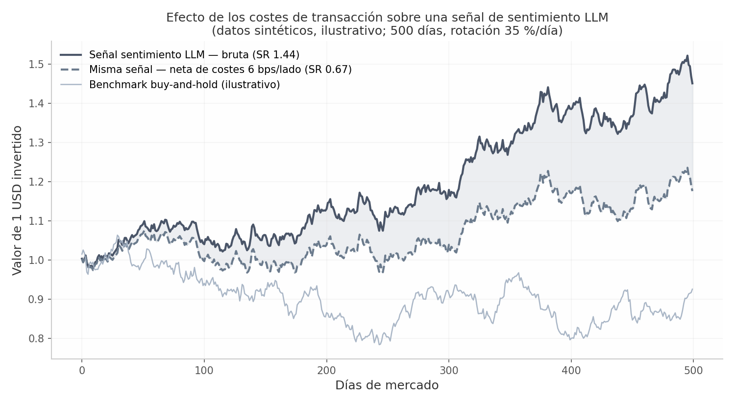
Figure 9.1. Gross (1.44) versus net (0.67) Sharpe of a synthetic sentiment signal with 6 bps per side and 35% daily turnover. Own elaboration with synthetic data, Jul-2026.
# --- Almgren-Chriss: optimal liquidation trajectory ---
import numpy as np

def almgren_chriss_trajectory(X, T, N, sigma, eta, lam):
    tau = T / N
    kappa = np.sqrt(lam * sigma**2 / eta)           # urgency κ ≈ sqrt(λσ²/η)
    t = np.arange(N + 1) * tau
    x = X * np.sinh(kappa * (T - t)) / np.sinh(kappa * T)
    return t, x, -np.diff(x), kappa                 # sales n_j per interval

t, x, n, k = almgren_chriss_trajectory(1e6, T=1.0, N=390,
                                       sigma=0.02, eta=1e-7, lam=1e-6)
print(f"Vida media de la liquidación θ=1/κ = {1/k:.3f} días")

# --- Total cost in bps: spread + sqrt impact + borrow ---
def coste_total_bps(Q, V_dia, sigma_dia, spread_bps, comision_bps,
                    Y=0.6, r_borrow=0.0, dias_corto=0, direccion=1):
    impacto = Y * sigma_dia * np.sqrt(Q / V_dia) * 1e4
    borrow  = r_borrow / 360 * dias_corto * 1e4 if direccion < 0 else 0.0
    return 0.5 * spread_bps + impacto + comision_bps + borrow
FINSABER provides the empirical verification at scale: in systematic backtests over two decades and more than 100 symbols, the advantages of timing-based LLM strategies deteriorate significantly relative to the reported narrow windows, and the regime analysis shows the perverse pattern of excess caution in bull markets and excess aggression in bear markets (arXiv.org) . The following table condenses the validation checklist that an institutional allocation committee demands before real capital.
Table 9.3 — Institutional strategy-validation checklist before allocating real capital
| # | Checkpoint | Minimum standard |
|---|---|---|
| 1 | Full costs | Commissions, spread, calibrated slippage, impact (√ or Almgren–Chriss), borrow, taxes (Blockchain News) |
| 2 | Point-in-time data | Universes with delistings; fundamentals with real publication date (臺灣博碩士論文知識加值系統) |
| 3 | Strict OOS validation | Anchored/rolling walk-forward; CPCV with purge + embargo (arXiv.org) |
| 4 | Selection correction | Reported N trials; DSR > 0.95 or Harvey–Liu haircut; PBO via CSCV (PyPI) |
| 5 | LLM anti-leakage discipline | Post-cutoff backtest only; counterfactual tests; random baseline (arXiv.org) |
| 6 | Modeled ingestion lag | Availability timestamps, not publication ones (horizontrading.io) |
| 7 | Extended paper trading | ≥ 3–6 months; realized vs. assumed slippage; pre-registered parity criterion (ResearchGate) |
| 8 | Pre-trade controls | Deterministic RiskGateway, kill switch, HITL, audit trail (15c3-5 floor) (skywork.ai) |
| 9 | Capacity | Maximum AUM before concave impact eats the alpha (🦜️🔗 LangChain) |
| 10 | Reproducibility and gradual deployment | Code, data, and seeds; paper → micro-capital → scaling with continuous TCA (LangChain) |
Interpretation. The checklist is not bureaucracy: each point neutralizes a failure mode documented in the literature reviewed in section 9.1. Points 1–4 are the classic standard any allocator would already demand of a traditional quant manager; points 5–6 are the LLM-era addition, because parametric leakage and the publication/availability gap are look-ahead channels with no classic analog that code inspection cannot rule out (horizontrading.io) . Point 7 operates as a time trial by fire: a signal with real edge degrades smoothly in paper trading, while a backtest artifact collapses within weeks. Points 8–10 connect with section 9.4 and with modules 10 and 12 of the course, where the RiskGateway and this checklist are formalized as capstone deliverables. The final decision rule is binary: if any of the ten points cannot be verified, the strategy receives no capital — regardless of how impressive the gross equity curve looks.
In plain terms: the square-root law and the invisible rent on shorts
The square-root law says something counterintuitive but empirically robust: moving twice the size does not cost twice as much, it costs \(\sqrt{2} \approx 1{,}41\) times more — and the module's mnemonic makes it tangible: trading one day of volume costs approximately one day of volatility. Think of crossing a river: if your order is a glass of water, the riverbed barely notices; if it is comparable to the daily flow, you are the one moving the water level. That is why impact is irrelevant for a small portfolio and, at the same time, is the capacity limit of any strategy that scales: the alpha left over at USD 1 M may not exist at USD 500 M, not because the signal deteriorates, but because your own execution eats it.
The second forgotten cost is borrow: selling short is renting the shares, and the rent is paid daily (\(r_b/360\) per day on the position's value). A general collateral ETF like SMH quotes at 0.7% annual, but a hard to borrow name exceeds 10–100% — and remember the Lopez-Lira & Tang asymmetry: the short leg contributed triple the long leg (29 versus 9 bps/day). Omitting borrow in the backtest of a sentiment signal is not a minor simplification: it is omitting the main cost of the alpha source.
The double erosion, in figures: trials and turnover
The two forces separating a pretty backtest from a real strategy fit in one chart. On the left, the DSR of the module's example (Sharpe 1.2 annual, 3 years daily, skewness −1, kurtosis 6) as a function of the number of tested configurations: the institutional 0.95 threshold is lost already between 2 and 3 trials. On the right, the annual cost drag by bps per side and daily turnover: with full turnover, 5 bps per side is ~25 percentage points per year (\(250 \times 2 \times 5\) bps), and with the 35% turnover of Figure 9.1, 6 bps per side explain the drop from Sharpe 1.44 to 0.67.
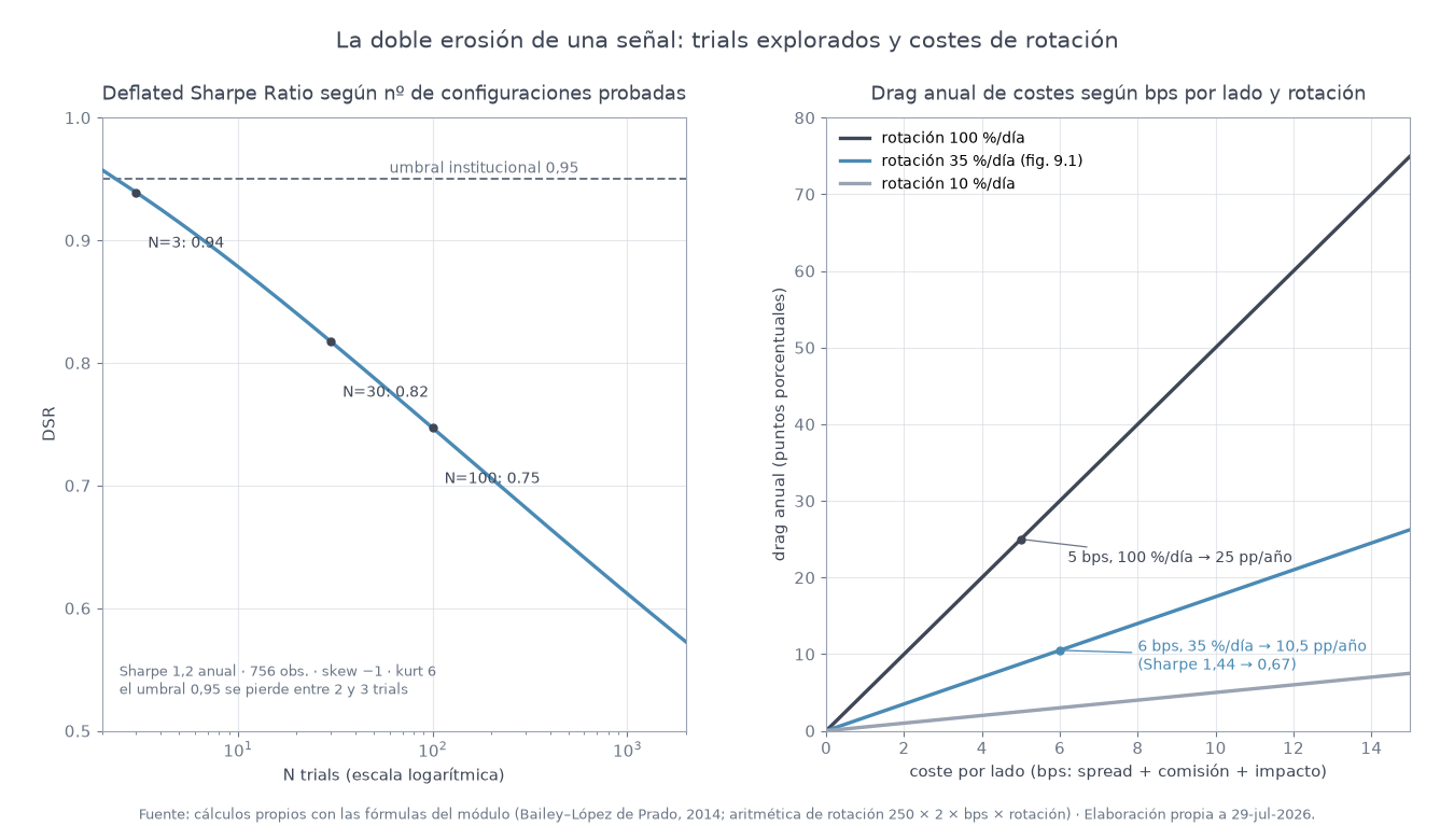
Figure 9.2. Left: Bailey–López de Prado DSR for a Sharpe of 1.2 (skew −1, kurt 6, 756 obs.) by N trials; the 0.95 threshold is crossed between 2 and 3 configurations. Right: annual drag in percentage points by bps per side for daily turnover of 10%, 35%, and 100%. Own elaboration with the module's functions, Jul-2026.
The joint reading is the module's thesis: a high-turnover signal needs a very high gross Sharpe to survive costs, and a high Sharpe obtained by extensive exploration needs a DSR that almost never survives honest trial accounting.
9.4 From signal to governed execution
9.4.1 Brokers, protocols, and the RiskGateway + HITL architecture
In the retail-prosumer world, Alpaca offers a commission-free REST/WebSocket API with a paper environment identical to live, 4x intraday / 2x overnight buying power, short selling, and advanced orders (bracket, OCO, trailing stop); the standard idempotency practice is the unique client_order_id, which prevents duplicating orders if the agent retries after a timeout (LangChain) . Interactive Brokers is the institutional-retail reference (global multi-asset access, public borrow feed (CSDN博客) ), and the current Python stack is ib_async, the maintained successor of ib_insync (archived) (LangChain) :
from ib_async import *

ib = IB()
ib.connect('127.0.0.1', 7497, clientId=1)          # 7497 = TWS paper

contract = Stock('TSLA', 'SMART', 'USD')
parent = LimitOrder('BUY', 100, 250.00)
parent.orderId = ib.client.getReqId(); parent.transmit = False
stop = StopOrder('SELL', 100, 240.00)
stop.orderId = ib.client.getReqId(); stop.parentId = parent.orderId; stop.transmit = False
tp = LimitOrder('SELL', 100, 260.00)
tp.orderId = ib.client.getReqId(); tp.parentId = parent.orderId; tp.transmit = True

for o in (parent, stop, tp):
    ib.placeOrder(contract, o)
In the institutional world the strategy does not talk to the broker: it talks to the OMS (order lifecycle, compliance, allocation, audit —the system of record), which routes to the EMS (smart order routing, VWAP/TWAP/IS algos, TCA), which executes against venues via FIX (langchain.com) . FIX 4.2 remains massively deployed for equities: SOH-delimited tag=value messages, with 35=D NewOrderSingle, 35=8 ExecutionReport, 35=F OrderCancelRequest and 35=G Cancel/Replace, session with Logon (35=A) and Heartbeat (35=0), and strictly monotonic sequence numbers (tag 34) —a gap triggers ResendRequest (35=2)— (arXiv.org) :
8=FIX.4.2|49=CLIENT|56=EXCHANGE|34=1|52=20260729-13:00:00|35=D|11=LLM-7F3A|55=AAPL|54=1|38=500|40=2|44=212.50|10=123|
The regulatory floor is SEC Rule 15c3-5 (Market Access Rule): after the Flash Crash, broker-dealers must apply automated and non-delegable pre-trade controls —capital and credit limits, maximum order size, prevention of erroneous orders and, for DMA, real-time monitoring and a kill switch— (skywork.ai) . The lesson for LLM systems is direct: the regulation assumes the algorithm will fail and mandates that the guardrail be independent of the order generator. The architecture taught in this course implements exactly that principle: the agent never has trading credentials; it has a submit_order tool wrapped in a deterministic RiskGateway (limits in code, never in the prompt), a HITL interrupt for orders above a threshold, and a kill switch that never asks for permission (🦜️🔗 LangChain) .
class RiskGateway:
    """Deterministic pre-trade risk layer (15c3-5 style)."""
    def __init__(self, api, max_notional=25_000, max_daily_loss=5_000, max_orders_min=10):
        self.api, self.max_notional = api, max_notional
        self.max_daily_loss, self.max_orders_min = max_daily_loss, max_orders_min
        self.kill = False                      # global kill switch

    def check(self, symbol, qty, price, side):
        if self.kill:
            raise RiskBlock("KILL-SWITCH ACTIVO: toda nueva orden bloqueada")
        if qty * price > self.max_notional:
            raise RiskBlock(f"Notional {qty*price:.0f} > límite {self.max_notional}")
        if self.daily_realized_pnl() < -self.max_daily_loss:
            self.kill = True                   # auto-kill on daily loss
            self.cancel_and_flatten()
            raise RiskBlock("Límite de pérdida diaria: posiciones cerradas")
        if self.orders_last_minute() >= self.max_orders_min:
            raise RiskBlock("Rate limit interno excedido (anti runaway-loop)")
        if side == "sell" and not self.is_shortable(symbol):
            raise RiskBlock(f"{symbol} no shortable / borrow no disponible")
        return True

class RiskBlock(Exception): pass
The LangChain integration uses HumanInTheLoopMiddleware: it interrupts execution at configured tool calls, persists state with a checkpointer, and admits approve/edit/reject/respond decisions, with conditional interrupts (when) to require human approval only above a given notional (🦜️🔗 LangChain) :
from langchain.agents import create_agent
from langchain.agents.middleware import HumanInTheLoopMiddleware, ToolCallRequest

def big_order(request: ToolCallRequest) -> bool:
    a = request.tool_call["args"]
    return a.get("qty", 0) * a.get("limit_price", 0) > 10_000   # conditional HITL

agent = create_agent(
    model="gpt-5.5",
    tools=[get_market_data, compute_signal, submit_order, cancel_all_orders],
    middleware=[HumanInTheLoopMiddleware(
        interrupt_on={
            "submit_order": {"allowed_decisions": ["approve", "reject"], "when": big_order},
            "cancel_all_orders": False,      # the kill switch NEVER asks for permission
            "get_market_data": False,
        },
        description_prefix="ORDEN PENDIENTE DE APROBACIÓN",
    )],
    checkpointer=AsyncPostgresSaver(...),      # mandatory for HITL
)

The kill-switch triggers are concrete and monitorable: daily loss, deviation of realized slippage from that assumed in the backtest, anomalous latency, data errors (gaps, future timestamps), LULD halts, or the operator's manual button. The FIX equivalent is a mass 35=F followed by session logout (35=5). The module's honest closing metric is therefore unique: the Sharpe net of costs, deflated by the N trials, validated post-cutoff, and executed under 15c3-5-style controls. Everything else is backtest marketing.
Common pitfall: the decorative HITL
A badly designed human-in-the-loop gives a false sense of control and no real one. Three failure modes documented in practice:
- Approval fatigue. If the threshold fires on every order, the operator ends up mechanically approving in seconds what they should review in minutes; the interrupt exists, but the judgment is gone. The
whenthreshold must fire rarely — that is what the RiskGateway is for, absorbing the routine case. - Algorithmic smurfing. With a HITL that fires above USD 10,000 of notional per order, an agent wanting to buy USD 60,000 learns to split it into six orders of 9,999. The defense is not in the prompt but in the gateway: aggregating notional per symbol and time window (the
max_orders_minand the daily limits of the module'sRiskGatewayare exactly that). - A kill switch that asks permission. If canceling everything requires human approval, it is not a kill switch: it is a suggestion. That is why in the module's code
cancel_all_ordershasinterrupt_on: False— the spirit of SEC 15c3-5 is that the guardrail be independent of the order generator, precisely because the regulation assumes the algorithm will fail.
The trial by fire is simple: simulate in paper an agent in a loop issuing 200 orders per minute (module exercise 5) and count how many the human reviewed with judgment. If the answer is embarrassing, the HITL was decorative.
The lifecycle of a governed order
The module's diagram shows the static architecture; this sequence shows the temporal dynamics — where state is persisted, where the human enters, and what travels over FIX in each direction:
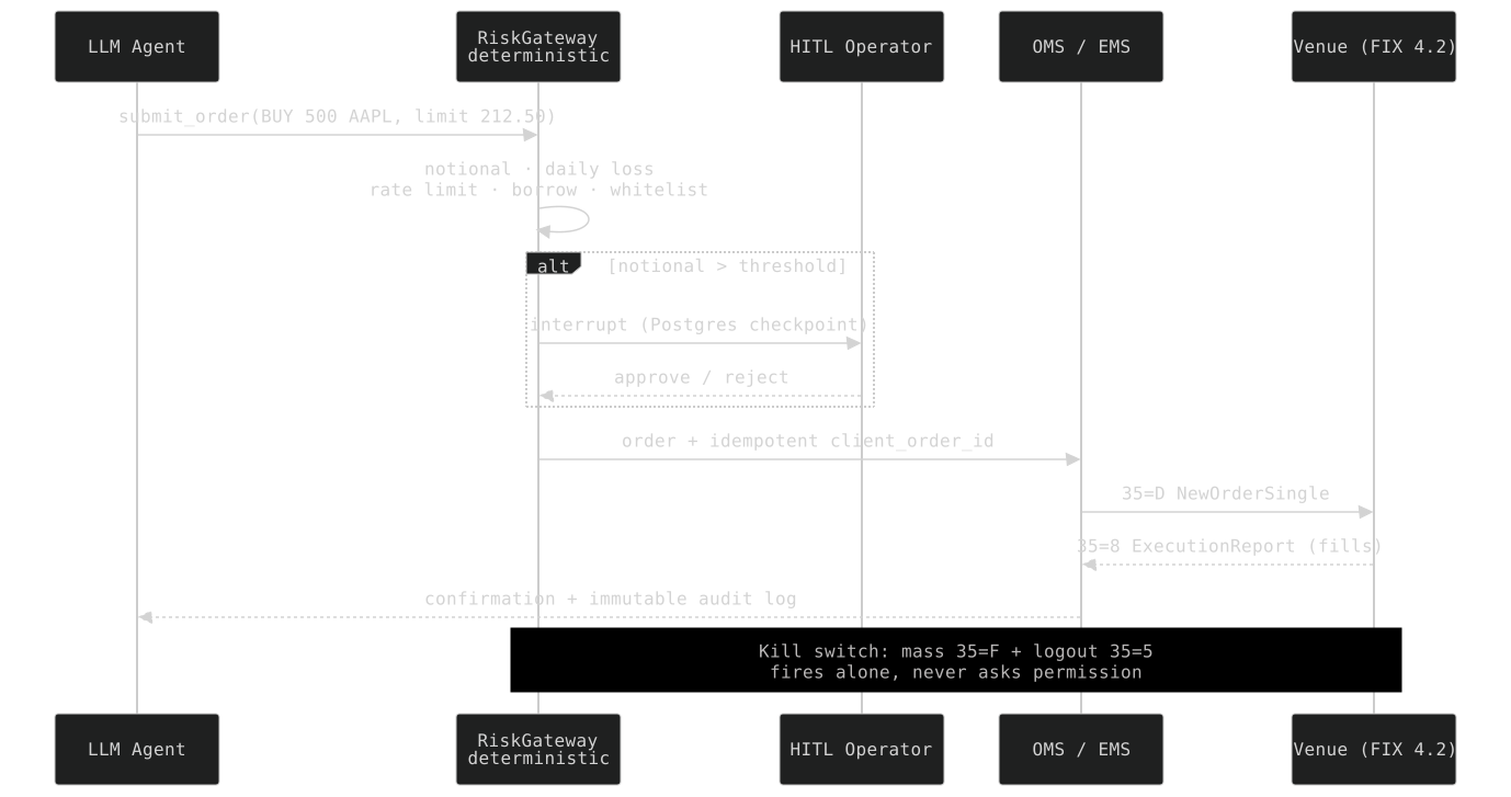
Two details that matter in production: the client_order_id makes the retry after a timeout idempotent (without it, the same order is duplicated), and FIX sequence numbers (tag 34) are monotonic — a gap triggers ResendRequest (35=2), so the session and its state are also part of the risk system.
Exercises
- Sentiment-signal backtest with vectorbt. Build a synthetic signal of LLM scores over 50 tickers (or download real headlines and score them with a model via batch API), aggregate it with a 2-day half-life decay, and turn it into long-only entries/exits of the top quintile. Run
Portfolio.from_signalswithfees=0, slippage=0and withfees=0.001, slippage=0.001; report gross Sharpe, net Sharpe, and implied turnover. Repeat withfees=0.003and discuss at what friction level the signal ceases to be viable. - DSR calculation. Using the module's
probabilistic_sharpe,expected_max_sharpe, anddeflated_sharpefunctions, take the net Sharpe from exercise 1 and compute the DSR assuming N ∈ {1, 10, 100, 1,000} trials, with the sample skewness and kurtosis of your returns. From what N does the DSR fall below 0.95? Compare with the Harvey–Liu haircut for 100 tests. - Almgren–Chriss cost simulation. Liquidate 1,000,000 shares in one day (390 1-minute intervals) with σ = 0.02, η = 10⁻⁷ and λ ∈ {10⁻⁷, 10⁻⁶, 10⁻⁵}. Plot the three trajectories \(x_j\), compute the half-life θ = 1/κ of each, and numerically verify the TWAP limit when κT ≪ 1. Then estimate the impact cost with the square-root law for Q/V_D ∈ {1%, 5%, 25%} and Y = 0.6.
- Turnover arithmetic. A sentiment strategy turns over 100% of the portfolio daily, half in shorts on small-caps with a 12% annual borrow. Compute the total annual drag with 8 bps per side of friction (spread + commission) and the daily borrow of the short leg. What minimum gross Sharpe does the signal need for a net Sharpe of 1.0, assuming 15% annual volatility?
- RiskGateway design. Extend the module's
RiskGatewayclass with: (a) a per-sector concentration limit; (b) a volume participation limit (≤ 10% of the symbol's ADV, estimated with the square-root law); (c) a symbol whitelist; (d) auto-kill if the average realized slippage of the last 50 orders exceeds 2× that assumed in the backtest. Write the unit tests proving that no order can reach the broker bypassing a limit, including the case of an agent in a loop issuing 200 orders per minute. - Paper audit. Choose one of the papers from the table in section 9.1.1 and evaluate it against the 10 points of the institutional checklist: identify which points it satisfies, which it violates, and what minimum additional experiment would be needed for its results to be admissible before an allocation committee. Present your conclusions in one page in the format evidence → rule → conclusion.
Module 9 of 15 — LangChain for Quantitative Trading. Data and versions verified as of July 2026; prices and market figures subject to change. LangChain 1.3.14 / langchain-core 1.5.2.
Elite resources to go deeper
- Lopez-Lira & Tang — Can ChatGPT Forecast Stock Price Movements? (arXiv 2304.07619): the LLM signal with the best evidence; read the version history — GPT-4's Sharpe went from 3.8 (v4) to 3.28 (v5), a lesson in fragility in itself.
- Bailey, Borwein, López de Prado & Zhu — The Probability of Backtest Overfitting (arXiv 1401.0478): the full CSCV/PBO framework, with the IS/OOS combinatorics summarized in section 9.3.1.
- Yu et al. — FinMem (arXiv 2311.13743): memory layered by time horizon; read it as an architecture pattern, not as a strategy.
- Yu et al. — FinCon (arXiv 2407.06567): manager–analyst hierarchy with verbal reinforcement and CVaR gating; notable for admitting memory hallucinations in the paper itself.
- SEC — Rule 15c3-5, Market Access Rule (final text, PDF): the primary source of the regulatory floor for pre-trade controls; the origin of the "the guardrail is not delegated" principle.
- FIX Trading Community — FIX standards: official specification of the tag=value protocol; for day-to-day work, the online FIX 4.2 dictionary is the quick reference for the
35=D/8/F/Gmessages. - nautilus_trader — documentation: the reference for the backtest→live parity pattern (same code, only the configuration changes) required by section 9.3.1.
- ib_async — official repository: the maintained successor of
ib_insyncfor Interactive Brokers; the current Python stack of the module's bracket-order example.
Check your understanding
Self-assessment with instant feedback. No scores are stored: it is just for you.