Quantitative risk: from VaR to the risk copilot
Exact VaR and Expected Shortfall, stress testing, and the LLM as an explanation layer, never a calculator.
Learning objectives
- Compute and interpret Value at Risk by the three standard methods (delta-normal, historical simulation, and Monte Carlo/FHS) and Expected Shortfall via the Rockafellar–Uryasev variational representation.
- Validate a VaR model with Kupiec's likelihood-ratio tests (POF) and Christoffersen's conditional coverage test, and relate them to the regulatory traffic light.
- Model volatility with RiskMetrics EWMA (\(\lambda = 0{,}94\)) and GARCH(1,1), including the \(k\)-step-ahead forecast with mean reversion.
- Select the appropriate performance ratio (Sharpe, Sortino, Omega, Calmar, Sterling, Ulcer Index) knowing their conventions and documented biases, in particular the overstatement of the Sharpe ratio under autocorrelation (Lo, 2002).
- Decompose portfolio risk with the Euler decomposition (Component/Marginal VaR) and design historical, hypothetical, and reverse stress testing programs in line with BCBS d450 and FRTB.
- Build a risk copilot with LangChain in which deterministic tools compute, the LLM narrates the attribution, and an
interruptescalates to the human — and justify why the LLM never computes the risk figure.
Modules 4 through 6 built the understanding layer: data sources, document RAG, and prompts with structured output. With this module the course enters Block III —reason and decide— and changes register: exact mathematics takes the lead here, and the LLM is confined to the role the golden rule assigns it (§1.2.2): narrate, orchestrate, and alert, never compute.
7.1 Risk measurement with exact formulas
Quantitative risk management rests on a small set of formulas whose provenance is verifiable: the J.P. Morgan/Reuters RiskMetrics Technical Document (1996), the Basel Committee documents (d450, d457), and the canonical academic literature (Rockafellar–Uryasev, Kupiec, Christoffersen, Bollerslev). This module presents them exactly as they appear in the primary sources, with the positive-loss convention: \(r_t\) denotes the log return on day \(t\); \(\alpha\) is the tail significance level (0.01 for 99% VaR); \(z_\alpha = \Phi^{-1}(1-\alpha)\) is the standard normal quantile of the right loss tail; \(\varphi\) and \(\Phi\) are the standard normal density and distribution function.
7.1.1 VaR, Expected Shortfall, and validation
Parametric VaR (delta-normal). Under normal returns, VaR at confidence \(1-\alpha\) and horizon \(h\) days for a portfolio of value \(V\) with daily mean \(\mu\) and daily volatility \(\sigma\) is (graphrag.com) :
with \(z_{0{,}05} = 1{,}645\) (95%) and \(z_{0{,}01} = 2{,}326\) (99%). Time scaling applies the square-root-of-time rule, \(\sigma(h) = \sigma\sqrt{h}\), valid only under i.i.d. returns. For a multi-asset portfolio with weights \(w\) and covariance matrix \(\Sigma\) (The Database for Multimodal AI) :
Numerical case. A portfolio of \(V = 100{,}000{,}000\) USD with \(\sigma = 1{,}1\%\) daily and \(\mu \approx 0\) has \(\mathrm{VaR}_{0{,}01}(1) = 100{,}000{,}000 \times 2{,}326 \times 0{,}011 = 2{,}558{,}600\) USD; over 10 days, \(\mathrm{VaR}_{0{,}01}(10) = 2{,}558{,}600 \times \sqrt{10} \approx 8{,}091{,}000\) USD. The method is fast and linear in the factors, but fails with non-linearities (options) and fat tails (graphrag.com) .
Historical VaR (historical simulation). The historical factor moves of the last \(T\) days (typically 250) are reapplied to the current portfolio and the hypothetical P&Ls are sorted \(L_{(1)} \le L_{(2)} \le \dots \le L_{(T)}\); VaR is the empirical quantile (arXiv.org) :
With \(T = 250\) and \(\alpha = 0{,}05\), the 95% VaR is the 13th worst day (\(0{,}05 \times 250 = 12{,}5\)). It requires no distributional assumptions and captures the sample tails, but at 99% with 250 days there are only about 2.5 tail observations, which produces high sampling variation and slow response to regime changes (arXiv.org) .
Monte Carlo VaR and FHS. \(N\) factor paths are simulated under a calibrated model (GBM, Student-t, GARCH), the portfolio is revalued, and the quantile of the simulated distribution is taken (arXiv.org) :
where \(\hat{F}_{L,N}\) is the empirical CDF of the \(N\) simulated losses. The Filtered Historical Simulation variant (Barone-Adesi, Bourgoin, and Giannopoulos) fits a GARCH(1,1), extracts the standardized residuals \(z_t = r_t/\sigma_t\), and simulates \(\tilde r = \hat\sigma_{t+1} z^{*}\) by resampling \(z^{*}\) with replacement; comparative evidence shows that normal Monte Carlo underestimates the left tail relative to FHS (arXiv.org) .
Expected Shortfall / CVaR. For a loss variable \(L\) with continuous CDF, VaR and ES are defined as (🦜️🔗 LangChain) :
Under normality a closed form exists:
At 99% the factor is \(\varphi(2{,}326)/0{,}01 \approx 2{,}665\); at 97.5%, \(\varphi(1{,}960)/0{,}025 = 0{,}0584/0{,}025 = 2{,}338\), the central figure in the FRTB design (§7.2). Unlike VaR, ES is a coherent measure in the sense of Artzner et al. (1999): it satisfies subadditivity, the property VaR violates (🦜️🔗 LangChain) . The Rockafellar–Uryasev (2000) variational representation turns CVaR estimation and optimization into linear programming (🦜️🔗 LangChain) :
with \((x)_+ = \max(x, 0)\); the minimizer \(c^{*}\) is VaR itself. The empirical estimator in historical simulation is simply the average of the \(\lfloor T\alpha \rfloor\) worst losses.
VaR backtesting. An unvalidated VaR model is an opinion. With the exception indicator \(I_t = \mathbf{1}\{L_t > \mathrm{VaR}_t\}\), Kupiec's (1995) proportion-of-failures test contrasts the observed rate \(N/T\) against the nominal \(p\) (CurvedTrading) :
Numerical case. With \(T = 250\) days, \(p = 0{,}01\), and \(N = 7\) exceptions (expected: 2.5), \(LR_{POF} \approx 5{,}50\), above the critical \(\chi^2_1(0{,}95) = 3{,}84\): the model is rejected at 5% (with \(N = 6\), \(LR_{POF} \approx 3{,}56\), just below the threshold). Christoffersen (1998) decomposes conditional coverage into \(LR_{cc} = LR_{uc} + LR_{ind} \sim \chi^2_2\), where the independence term uses the transition probabilities \(\hat\pi_{01} = n_{01}/(n_{00}+n_{01})\) and \(\hat\pi_{11} = n_{11}/(n_{10}+n_{11})\), detecting streaks of exceptions that Kupiec's test does not see (langchain.ac.cn) . Both tests are required by the Basel II/III internal models frameworks (langchain.ac.cn) .
In plain terms: the levee, the flood, and the inspector
Think of a portfolio as a city next to a river. 99% VaR is the height of a levee that is overtopped only one year in a hundred: it tells you where the edge is, but nothing about what lies beyond it. Expected Shortfall answers the question the levee does not —"when it is overtopped, how much water comes in?"—: it is the average depth of the flood in the bad years, not its frequency. That is why two portfolios with the same VaR can hide very different floods, and why FRTB computes capital with ES.
The Kupiec test is the levee inspector: if the levee is overtopped seven times in 250 years when it promised 2.5, there is no need to argue about hydrology — the levee is undersized. And the Christoffersen test adds the fine nuance: seven floods spread at random is not the same as seven in a row; streaks reveal that the model is missing something persistent.
7.1.2 Volatility: the raw material of every risk number
Realized volatility. With \(M\) evenly spaced intraday observations of the log price and returns \(r_{t,i} = p_{t,i} - p_{t,i-1}\) (QVeris AI) :
Under a diffusion with jumps, \(RV_t\) is a consistent estimator of quadratic variation as \(M \to \infty\) (Andersen–Bollerslev); with microstructure noise, the practical optimal frequency is 5 minutes (QVeris AI) .
EWMA / RiskMetrics. The recursion from the RiskMetrics Technical Document (4th ed., 1996) is (graphrag.com) :
Expanded, \(\sigma_t^2 = (1-\lambda)\sum_{i=1}^{\infty}\lambda^{i-1} r_{t-i}^2\): decaying geometric weights with effective memory \(\approx 1/(1-\lambda) \approx 17\) days for \(\lambda = 0{,}94\). It is an IGARCH with no mean reversion (\(\omega = 0\), \(\alpha+\beta = 1\)), and its multivariate version \(\Sigma_t = \lambda\Sigma_{t-1} + (1-\lambda)\, r_{t-1} r_{t-1}^{\top}\) is always positive semidefinite (graphrag.com) .
In institutional practice. Three decades after its publication, \(\lambda = 0{,}94\) remains the de facto standard for daily volatility on risk desks: the RiskMetrics Technical Document (J.P. Morgan/Reuters, Dec-17-1996, now distributed by MSCI) set that parameter and the industry inherited it as the starting point of nearly every parametric VaR engine (graphrag.com) . The original document itself warned that "no amount of analytical sophistication will replace experience and professional judgment in risk management" (Godel Discount) — a 1996 sentence that precisely describes this module's governing principle for LLM copilots. At the most recent end, FinCon (NeurIPS 2024) uses the CVaR of the worst 1% of daily P&L as a gating signal that changes the manager agent's behavior (Github) : the tail metric decides, the language model narrates.
GARCH(1,1). The Engle (1982) and Bollerslev (1986) model introduces mean reversion (Bright Data) :
The unconditional variance (long-run level) is \(\bar\sigma^2 = \dfrac{\omega}{1-\alpha-\beta}\), and the \(k\)-step-ahead forecast reverts geometrically toward it:
The sum \(\alpha+\beta\) measures the persistence of volatility shocks; EWMA is the limiting case \(\omega = 0\), \(\alpha+\beta = 1\) (Bright Data) . Numerical case. With \(\alpha+\beta = 0{,}97\), a volatility spike that doubles the long-run level (\(\sigma_{t+1}^2 = 2\bar\sigma^2\)) takes \(k \approx \ln(0{,}5)/\ln(0{,}97) \approx 23\) days to reduce the excess by half.
Maximum drawdown and recovery asymmetry. Let \(V_t\) be the equity curve and \(\overline{V}_t = \max_{s\le t} V_s\) the running maximum; the drawdown is \(D_t = (V_t - \overline{V}_t)/\overline{V}_t \le 0\) and (Investopedia) :
Recovery is asymmetric: a loss \(d\) requires a gain \(g = \dfrac{d}{1-d}\) to return to the peak — a 50% drop demands a 100% rise, and a 90% drop, a 900% one (Investopedia) . It is the risk metric investors actually feel, and the one anchoring the Calmar and Sterling ratios.
In plain terms: volatility comes in clusters (and has a short memory)
Volatility is not dealt out like coin flips: turbulent days cluster with turbulent days and calm ones with calm ones. That clustering is exactly what the i.i.d. normal ignores and what EWMA and GARCH capture. EWMA is an average with a deliberately short memory: with \(\lambda = 0{,}94\) the most recent day weighs 6% and the effective memory is about 17 days — it reacts fast to a regime change, at the price of "forgetting" that a long-run level exists (it is an IGARCH: shocks do not revert). GARCH(1,1) adds exactly that: a gravity pulling variance toward \(\bar\sigma^2\). With \(\alpha+\beta = 0{,}97\), a spike that doubles the long-run level takes about 23 days to deflate by half (the module's calculation). Practical rule: EWMA to react, GARCH to project \(k\) steps ahead.
Recovering from a drawdown is not symmetric
Losing 20% is not fixed by gaining 20%: it is fixed by gaining 25%. Recovery requires \(g = d/(1-d)\), a convex function that explodes as soon as the drop grows larger — the module fixes the extremes: \(-50\%\) requires \(+100\%\) and \(-90\%\) requires \(+900\%\). It is the arithmetic reason why drawdown-anchored ratios (Calmar, Sterling, Ulcer Index) punish deep losses so hard, and why position sizing matters more than accuracy: recovery time grows faster than the loss.
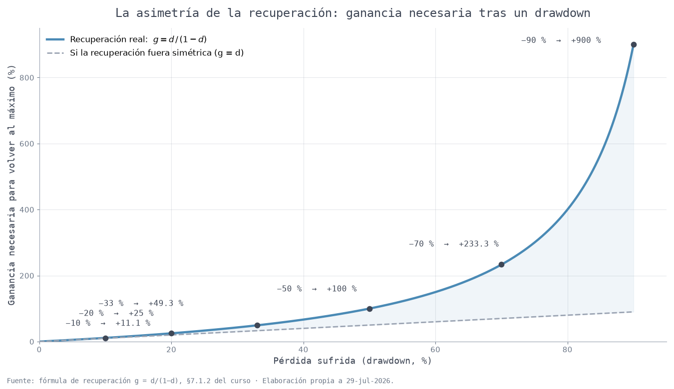
Figure 7.A. The curve \(g = d/(1-d)\) against the symmetric diagonal: beyond 30% drops the required recovery takes off violently. Own elaboration.
7.1.3 Risk-adjusted performance ratios
The full catalog, with its conventions and documented pitfalls:
Sharpe. Introduced as the reward-to-variability ratio (Sharpe, 1966) (AlphaLog) :
Annualization with \(\sqrt{12}\) or \(\sqrt{252}\) requires i.i.d. returns; with positive serial autocorrelation — typical of hedge fund strategies with smoothed valuations — the annualized Sharpe can be overstated by up to 65% (Lo, 2002) (Alpha Vantage) . It is the most ignored methodological warning in the industry.
Sortino. It replaces total volatility with the downside deviation relative to the minimum acceptable return \(\tau\) (canvasbusinessmodel.com) :
Omega (Keating–Shadwick, 2002). It uses the entire distribution, with no moment assumptions (canvasbusinessmodel.com) :
with empirical form \(\hat\Omega(\theta) = \dfrac{\frac{1}{n}\sum_{i=1}^n (R_i-\theta)^{+}}{\frac{1}{n}\sum_{i=1}^n (\theta-R_i)^{+}}\) (Macroption) .
Calmar. \(\mathrm{Calmar} = \dfrac{\mathrm{CAGR}}{|\mathrm{MDD}|}\), typically over 36-month windows; introduced by Terry W. Young (1991) (quantvps.com) . Window bias: a track record that has not yet lived through its crisis exhibits an artificially high Calmar (quantvps.com) .
Sterling. Deane Sterling Jones's (1981) original definition is (Alpha Vantage) :
with \(APR\) the compound annual return and \(ALD\) the average of the annual maximum drawdowns. The 10% reflected T-bill yields in 1981; variants with \(-10\%\) and modern versions with \(R_f\) coexist (langfuse.com) . Editorial rule: always cite the convention used.
Ulcer Index (Martin & McCann, 1987). Root mean square of percentage drawdowns from the last peak (TrueFoundry) :
The square penalizes the depth and the duration of drawdowns jointly; it is the basis of the Ulcer Performance Index, \(UPI = (R_p - R_f)/UI\) (TrueFoundry) .
Tracking error and information ratio. For an active portfolio against its benchmark \(b\) (🦜️🔗 LangChain) :
Grinold's (1989) fundamental law of active management decomposes IR into skill and breadth: \(IR \approx IC \cdot \sqrt{BR}\), where \(IC\) is the information coefficient (correlation between forecast and realization) and \(BR\) the number of independent bets (NextFuture) .
Higher-order moments and modified VaR. Equity returns exhibit negative skewness and excess kurtosis (kosmoy.com) :
(normal: \(S = 0\), \(K = 3\)). The Cornish–Fisher expansion (Zangari, 1996) corrects the Gaussian quantile (AgenticWire) :
and Boudt, Peterson, and Carl (2008) extend the correction to a coherent modified ES, \(\mathrm{ES}_{\mathrm{mod}} = \sigma\frac{\varphi(z)}{\alpha}\left[1 + \frac{z}{6}S + \frac{z^2-1}{24}K_{\mathrm{exceso}}\right] - \mu\) (AgenticWire) . The expansion stops being monotonic for \(|S| \gtrsim 2\) or \(K \gtrsim 6\): verify the monotonicity of \(z_{CF}\) in \(\alpha\) before reporting it (AgenticWire) .
The following table summarizes the module's main risk metrics.
Table 7.1 — Risk metrics: formula, horizon, assumptions, and main limitation
| Metric | Summary formula | Typical horizon | Key assumptions | Main limitation |
|---|---|---|---|---|
| Delta-normal VaR | \(V z_\alpha \sigma \sqrt{h}\) | 1–10 days | Normality, i.i.d., linearity | Underestimates fat tails and non-linearities (graphrag.com) |
| Historical VaR | \(L_{(\lceil T(1-\alpha)\rceil)}\) | 1 day (250 obs.) | History represents the future | ~2.5 tail obs. at 99%; slow under a new regime (arXiv.org) |
| Monte Carlo VaR / FHS | \(\hat F^{-1}_{L,N}(1-\alpha)\) | 1–10 days | Well-calibrated factor model | Specification risk; revaluation cost (arXiv.org) |
| ES / CVaR | \(\frac{1}{\alpha}\int_0^\alpha \mathrm{VaR}_u\,du\) | 1–10 days | Well-estimated tail | Statistically difficult backtesting (kosmoy.com) |
| EWMA RiskMetrics | \(\lambda\sigma_{t-1}^2 + (1-\lambda)r_{t-1}^2\) | Daily | \(\lambda = 0{,}94\) universal | No mean reversion (IGARCH) (graphrag.com) |
| GARCH(1,1) | \(\omega + \alpha\varepsilon^2 + \beta\sigma^2\) | Daily–monthly | Stationarity, \(\alpha+\beta<1\) | Persistence misestimated in crises (Bright Data) |
| MDD | \(\min_t (V_t - \overline V_t)/\overline V_t\) | Full history | Faithful equity curve | Window-dependent; backward-looking (Investopedia) |
Interpretation. No row of the table is dominant: each metric encodes a different assumption about where risk resides. Delta-normal VaR compresses the whole distribution into two parameters and is unbeatable in speed and analytical attribution (§7.2.1), but its price is normality; historical simulation gives up the distributional assumption in exchange for depending on a single past path, with barely 2.5 effective observations in the 99% tail over 250 days. ES corrects VaR's blindness to tail severity and is coherent (subadditive), but its statistical validation is harder — which is why FRTB computes capital with ES and backtests with VaR. Conditional volatility measures (EWMA, GARCH) feed all of the above: a calibration error in \(\sigma\) propagates linearly into VaR. MDD, finally, is not a probabilistic but a historical measure, and therefore complements — does not replace — tail measures: it answers the investor's question ("how much can I come to suffer, and for how long?") that no quantile answers.
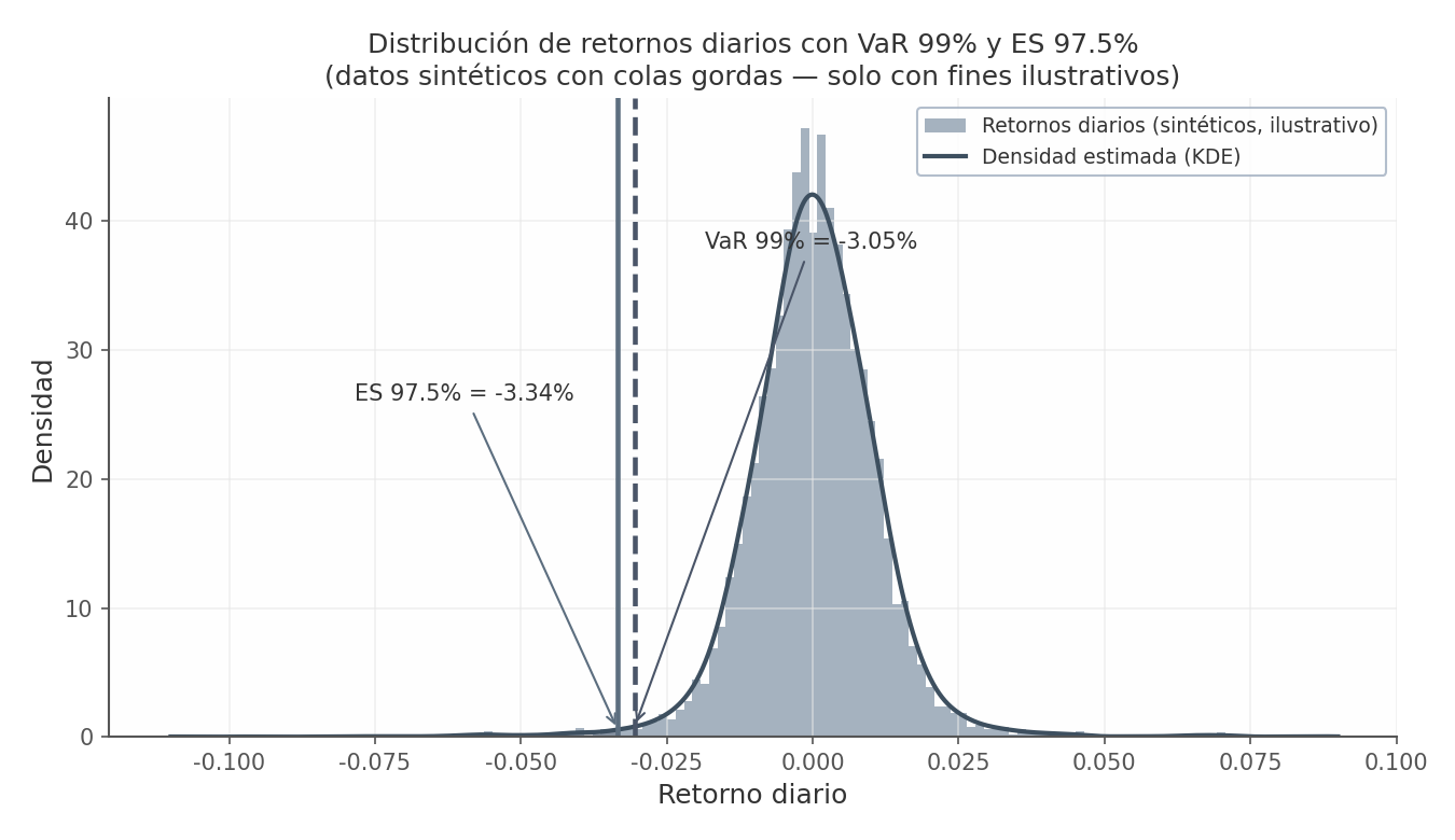
Figure 7.1. Synthetic daily returns distribution with fat tails (normal / Student-t mixture), with 99% VaR and 97.5% ES marked. With tails heavier than normal, ES pulls away from VaR into the tail: exactly the behavior FRTB seeks to capitalize. Data generated for purely illustrative purposes. Own elaboration, Jul-2026.
Common pitfall: annualizing Sharpe with \(\sqrt{252}\) and looking away
The rule \(S_{\mathrm{anual}} = S_{\mathrm{diario}}\sqrt{252}\) is only valid with i.i.d. returns, and almost nobody checks that assumption before applying it. The worst documented case is strategies with smoothed valuations (hedge funds with illiquid assets marked by hand): smoothing creates artificial positive autocorrelation, which at once inflates the apparent numerator of stability and, according to Lo (2002), can overstate the annualized Sharpe by up to 65% (§7.1.3). It is the most ignored methodological warning in the industry because the bias always plays in the manager's favor.
Three practical defenses: test serial autocorrelation (a Ljung–Box test or the Lo–MacKinlay variance ratio) before annualizing; recompute the Sharpe with de-smoothed returns or at longer horizons; and be editorially suspicious of any annualized monthly Sharpe from an illiquid strategy that does not document its valuation scheme.
7.2 Portfolio risk and stress testing
7.2.1 Euler decomposition, scenarios, and FRTB
Component and Marginal VaR. With parametric VaR \(\mathrm{VaR}_p = z_\alpha \sigma_p V\) and monetary positions \(x_i\), Garman's (1996) decomposition is (The Database for Multimodal AI) :
equivalently, \(\mathrm{CVaR}_i = \mathrm{VaR}_i \cdot \rho_{i,p}\). The Euler property guarantees exact aggregation: \(\sum_i \mathrm{CVaR}_i = \mathrm{VaR}_p\) (kosmoy.com) . Marginal VaR identifies the "worst hedge": the position with the highest MVaR is the one whose reduction cuts the most risk per monetary unit. This decomposition is, moreover, the mathematical basis of narrative risk attribution with an LLM (§7.3): the tool computes the \(\mathrm{CVaR}_i\), the language model explains them (The Database for Multimodal AI) . The underlying diversification is Markowitz's: with two assets, \(\sigma_p^2 = w_A^2\sigma_A^2 + w_B^2\sigma_B^2 + 2 w_A w_B \sigma_A \sigma_B \rho_{AB}\), and any \(\rho < 1\) reduces variance relative to the weighted average — with the critical caveat that in crises correlations converge to 1 (2008, March 2020) (confident-ai.com) .
Historical scenarios. The shocks observed in real episodes are reapplied to the current portfolio: subprime 2007-08, COVID March 2020, Black Monday 1987 (−22.6% for the Dow in a single session), LTCM 1998, the 2022 rates shock. For each factor, the worst 1-day and 10-day shocks are determined. Their value is that they preserve the real stress correlations: in 2008 developed-market equities fell together, and in March 2020 equities and Treasury bonds were sold simultaneously in the dash for cash (openobserve.ai) .
Hypothetical scenarios. Plausible extreme shocks not necessarily observed. A documented global bank's stress program combines historical scenarios ("subprime crisis", "Covid crisis") with a hypothetical worst case that moves each factor between ±3 and ±6 daily standard deviations, ignoring historical correlations (openobserve.ai) .
Reverse stress testing. The BCBS principles invert the logic: "a stress testing programme must determine what scenarios could challenge the bank's viability (reverse stress tests) and thereby uncover hidden risks and interactions between risks", starting "from a known stress outcome — a breach of regulatory capital ratios, illiquidity or insolvency — and asking what events could lead to that outcome" (BCBS 2009, p. 14) (Laminar) . PRA, EBA, and FCA incorporate it into their frameworks (ICAAP/SREP; FG 20/1), and the BCBS Range of Practices report (2017) documents that two-thirds of institutions practice it as a complement (xseek.io) . The 2018 Stress Testing Principles (BCBS d450) replace the 2009 ones and require stress testing as a mandatory complement to internal models, precisely to cover what the model's assumptions do not capture (kosmoy.com) .
FRTB: from 99% VaR to 97.5% ES. The Fundamental Review of the Trading Book (BCBS d352, 2016; revised in d457, 2019) replaces, in the internal models approach, 10-day 99% VaR with 97.5% ES calibrated over a stress period, with five liquidity horizons (10/20/40/60/120 days), a reduced set of modellable factors, and additive capital for non-modellable ones (NMRF) (kosmoy.com) . The calibration is deliberately continuous under normality (Holiday Landmark) :
— almost identical (\(2{,}338\sigma \approx 2{,}326\sigma\)) when returns are normal, but with ES growing much faster than VaR as soon as fat tails appear: "same number in calm times, a larger number precisely on the fat-tail exposures that VaR historically undercapitalized" (Holiday Landmark) . Backtesting is still done on 99% and 97.5% VaR with the traffic light over 250 days — because ES is not classically elicitable and its direct validation is statistically harder — complemented by the P&L Attribution Test (PLAT) at desk level; a desk that fails backtesting or PLAT is forcibly migrated from the internal to the standardized approach (kosmoy.com) . Implementation calendar: EU (CRR3) January 2026, UK (PRA) January 2027, US pending (braintrust.dev) .
Table 7.2 — FRTB (IMA) versus the previous internal approach (Basel 2.5)
| Dimension | Previous framework (Basel 2.5, IMA) | FRTB (IMA, d457) |
|---|---|---|
| Capital metric | 99% VaR, 10 days (+ stressed VaR) | 97.5% ES, calibrated to a stress period (braintrust.dev) |
| Horizon | Uniform 10 days | 10/20/40/60/120 days by factor liquidity (kosmoy.com) |
| Risk factors | All modellable by default | NMRF with additive capital; reduced set ≥ 75% of total ES |
| Diversification | Full implicit | IMCC recognizes only 50% of the benefit (\(\rho = 0{,}5\)) |
| Validation | Traffic light on 99% VaR | Traffic light on 99% and 97.5% VaR + desk-level PLAT (kosmoy.com) |
| Consequence of failure | Capital multiplier | Forced migration of the desk to the standardized approach (kosmoy.com) |
| Entry into force | 2011 (Basel 2.5) | EU Jan-2026; UK Jan-2027; US pending (braintrust.dev) |
Interpretation. The reform surgically corrects VaR's three documented failures — non-subadditivity, blindness to tail severity, and procyclicality from calibration to low recent volatility (braintrust.dev) — without breaking operational continuity: the arithmetic \(2{,}338\sigma \approx 2{,}326\sigma\) guarantees that, in a normal world, capital barely changes, while in a fat-tailed world ES demands more precisely where VaR failed in 2008. The staggered liquidity horizons recognize that not all factors can be liquidated in 10 days, and the NMRF regime penalizes the opportunistic modelling of factors with scarce data. The decision to keep the traffic light on VaR — and not on ES — is a concession to statistics: ES is not elicitable in the classical sense, so validation stays with the quantile. For the quant reader, the practical lesson is that a modern risk engine must produce both families of numbers (VaR for validation, ES for capital) on the same scenario infrastructure.
Worked example: Component VaR in a two-position portfolio
A 100M USD portfolio with two positions: \(x_A = 60\) M in equities (\(\sigma_A = 1{,}2\%\) daily) and \(x_B = 40\) M in bonds (\(\sigma_B = 0{,}8\%\)), correlation \(\rho = 0{,}3\), 99% VaR (\(z = 2{,}326\)).
Step 1 — covariances. \(\Sigma_{AA} = 0{,}012^2 = 1{,}44\times10^{-4}\), \(\Sigma_{BB} = 0{,}008^2 = 6{,}4\times10^{-5}\), \(\Sigma_{AB} = 0{,}3 \times 0{,}012 \times 0{,}008 = 2{,}88\times10^{-5}\).
Step 2 — \((\Sigma x)\) in monetary terms. \((\Sigma x)_A = 1{,}44\times10^{-4}\cdot60\,\text{M} + 2{,}88\times10^{-5}\cdot40\,\text{M} = 8.640 + 1.152 = 9.792\); \((\Sigma x)_B = 1.728 + 2.560 = 4.288\).
Step 3 — portfolio VaR. \(\sigma_p = \sqrt{x^\top \Sigma x} = \sqrt{60\,\text{M}\times9.792 + 40\,\text{M}\times4.288} \approx 871.230\) USD; \(\mathrm{VaR}_p = 2{,}326 \times 871.230 \approx 2.026.480\) USD.
Step 4 — components. \(\mathrm{CVaR}_A = z \cdot x_A (\Sigma x)_A / \sigma_p \approx 1.568.550\) USD (77.4%); \(\mathrm{CVaR}_B \approx 457.930\) USD (22.6%).
Step 5 — Euler check. \(1.568.550 + 457.930 \approx 2.026.480 = \mathrm{VaR}_p\): aggregation is exact, up to rounding. The desk reading: position A is 60% of the notional but 77.4% of the risk; cutting 1 USD of A removes about 2.6 cents of VaR versus 1.1 cents per USD of B. Marginal VaR, not weight, says where to cut.
import numpy as np

def euler_cvar(x: np.ndarray, cov: np.ndarray, z: float = 2.326) -> dict:
    """Parametric Component VaR with Euler aggregation check."""
    sx = cov @ x
    sigma_p = float(np.sqrt(x @ sx))
    var_p = z * sigma_p
    cvar = x * (z * sx / sigma_p)          # CVaR_i = x_i · MVaR_i
    return {"var_p": round(var_p, 2),
            "cvar": np.round(cvar, 2).tolist(),
            "pct": np.round(100 * cvar / var_p, 1).tolist(),
            "euler_check": round(float(cvar.sum() - var_p), 2)}  # ≈ 0.0
With x = [60e6, 40e6] and the cov from step 1 it returns pct = [77.4, 22.6] and euler_check ≈ 0. This JSON is exactly what an euler_attribution tool would hand to the copilot of §7.3: the tool computes the Component VaRs with their aggregation check, and the language model merely narrates them, quoting each figure exactly as received.
7.3 The risk copilot with LangChain
7.3.1 Canonical pattern: the tool computes, the LLM narrates, the human vetoes
The 2024-2026 literature documents a transition from "LLMs as text analysts" to LLM agents with quantitative tools: the LLM reasons and orchestrates; the numbers are computed by deterministic code (horizontrading.io) . The 2026 trading-agent taxonomy classifies risk control as a native capability of the agent — "risk as a gating mechanism in the action architecture, not post-hoc" (horizontrading.io) — and the reference case is FinCon (NeurIPS 2024): its intra-episode risk alert is triggered by a sudden drop in CVaR, defined as the mean of the worst 1% of daily P&L, and when activated "the manager agent adopts a risk-averse stance that day, regardless of the prior risk state" (Github) . In the open source ecosystem, MCP servers such as wraquant-mcp expose 218 tools (risk, volatility, and regime modules) to Claude/LangChain agents; the documented conversation pattern is literally "VaR(95%): −2.1%, CVaR: −3.4%" computed by the tool and narrated by the agent (quodfinancial.com) . LangChain also maintains an official sample repository of a risk assessment agent (langchain-samples/risk-assessment-agent, LangGraph + LangSmith) with GRC scenarios and human-in-the-loop (TS Imagine) , and projects such as DART architecturally separate risk_manager.py (Monte Carlo VaR, Kelly, sizing) from the LLM analyzer (sanj.dev) .
Layer 1: the deterministic tool. Every risk figure is produced in Python, with controlled rounding and structured output:
import numpy as np
from langchain_core.tools import tool

@tool
def compute_var_es(returns: list[float], confidence: float = 0.99) -> dict:
    """VaR and Expected Shortfall via historical simulation (positive losses)."""
    r = np.asarray(returns, dtype=float)
    losses = np.sort(-r)                       # positive losses, sorted
    alpha = 1.0 - confidence
    var = float(np.quantile(losses, confidence))
    tail = losses[losses >= var]
    es = float(tail.mean()) if tail.size else var
    # Controlled rounding: the LLM receives the final figure, never recomputes it
    return {"var": round(var, 6), "es": round(es, 6),
            "n_tail": int(tail.size), "alpha": alpha, "method": "historical"}
Layer 2: backtesting as a validation tool. The same principle applies to Kupiec's test:
import numpy as np
from scipy.stats import chi2
from langchain_core.tools import tool

@tool
def kupiec_pof(exceptions: int, n_days: int, p: float = 0.01) -> dict:
    """Kupiec POF test: H0 = the exception rate equals the nominal p."""
    N, T = exceptions, n_days
    lr = -2.0 * (np.log((1 - p) ** (T - N) * p ** N)
                 - np.log((1 - N / T) ** (T - N) * (N / T) ** N))
    return {"lr_pof": round(float(lr), 4),
            "p_value": round(float(chi2.sf(lr, 1)), 4),
            "reject_5pct": bool(lr > chi2.ppf(0.95, 1))}
Layer 3: the copilot agent with human escalation. The LLM orchestrates the tools and drafts the attribution based on the Euler decomposition it receives as JSON; an interrupt halts the flow on any limit breach so the risk manager decides:
from langchain.agents import create_agent
from langchain.agents.middleware import HumanInTheLoopMiddleware
from langgraph.checkpoint.memory import InMemorySaver

SYSTEM = (
    "Eres un copiloto de riesgo institucional. NUNCA calcules cifras de riesgo: "
    "usa SIEMPRE las herramientas compute_var_es, kupiec_pof y euler_attribution. "
    "Narra la atribución solo a partir del JSON que devuelvan las herramientas, "
    "citando cada número exactamente como lo recibiste."
)

copilot = create_agent(
    model="claude-sonnet-4-6",
    tools=[compute_var_es, kupiec_pof, euler_attribution],
    system_prompt=SYSTEM,
    middleware=[
        HumanInTheLoopMiddleware(
            interrupt_on={
                "escalate_limit_breach": True,   # approve / edit / reject / respond
                "compute_var_es": False,          # safe read
            },
        ),
    ],
    checkpointer=InMemorySaver(),  # in production: PostgresSaver (audit log)
)
The full architecture separates three planes of responsibility:

Diagram 7.1. Risk copilot architecture: deterministic tools produce every figure; the LLM narrates the Euler-based attribution; the interrupt escalates to the human on breaches.
Limit monitoring with natural-language alerts. A scheduler runs the VaR/ES/MDD computation against limits; on a breach, the agent composes the alert —which limit, by how much it is exceeded, which positions contribute according to Component VaR, suggested action— and the interrupt holds it until the human decision (TS Imagine) :

Diagram 7.2. Limit monitoring flow: detection is quantitative; the LLM provides the alert narrative; the human retains the decision.
from langgraph.types import interrupt

def breach_node(state):
    if state["var_99"] <= state["limit"]:
        return {"status": "compliant"}
    alert = llm.invoke(ALERT_PROMPT + json.dumps(state["euler_breakdown"]))
    decision = interrupt({"alert": alert, "state": state})  # pause until the human
    return {"status": decision["action"], "alert": alert}
Worked example: a limit breach, from the figure to the human veto
Let's walk through Diagram 7.2 with concrete numbers. At the close, the scheduler calls compute_var_es over 250 days of returns and receives the figure already fixed by the tool:
{"var": 0.0272, "es": 0.0341, "n_tail": 3, "alpha": 0.01, "method": "historical"}
The portfolio's 99% VaR amounts to 2.72M USD against a limit of 2.50M: a 220,000 USD breach. The graph's conditional edge routes the state to the alert node; the LLM also receives the euler_attribution breakdown (pct = [77.4, 22.6]) and drafts: "99% VaR of 2.72M USD, 220,000 USD above the limit; 77.4% of the risk comes from position A; reducing A by ~10M USD is suggested". Every number in the text matches the JSON — if not, the exact-match evaluation of exercise 4 would catch it. Then the interrupt pauses the graph:
decision = interrupt({"alert": alert, "var": 0.0272, "limit": 0.025,
                      "euler": {"A": 77.4, "B": 22.6}})
The risk manager reviews and resumes with their decision, which stays in the checkpoint as audit evidence:
from langgraph.types import Command

copilot.invoke(Command(resume={"action": "approve", "reduce_A": 10_000_000}),
               config={"configurable": {"thread_id": "limit-monitor-1"}})
The full flow, with the pause as a first-class citizen:
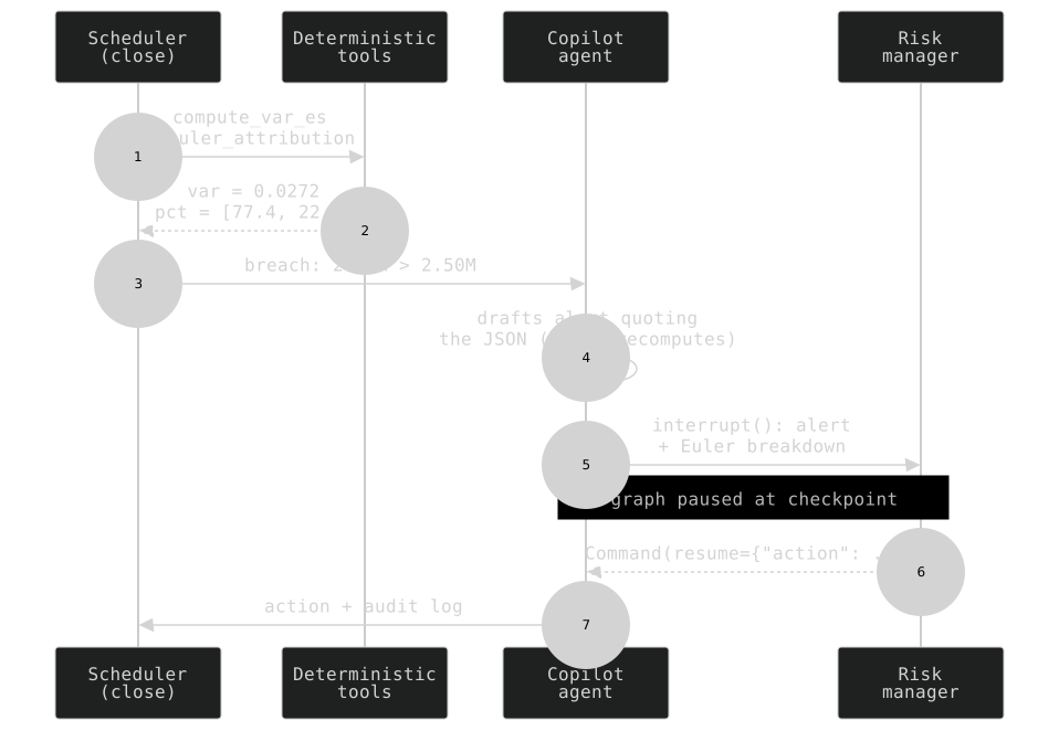
Notice what does not happen at any step: the LLM does not add, does not average, does not interpolate. The tool computes and rounds; the model narrates; the human decides.
7.4 The limits of the model and of the LLM
7.4.1 Structural critique of VaR, numerical hallucination, and model risk
The anti-VaR literature. Nassim Taleb campaigned against VaR for more than a decade and called it, literally, "a fraud" (NYT Magazine, Jan-4-2009); David Einhorn described it as "relatively useless as a risk-management tool and potentially catastrophic when its use creates a false sense of security… like an airbag that works all the time, except when you have an accident" (quodfinancial.com) . The quantification of the failure is brutal: under normality, a \(5\sigma\) event should occur once every ~14,000 years; equity markets produce such events roughly once per decade, and in 2008 books with "moderate" 99% VaR suffered losses of several times VaR (🦜️🔗 LangChain) . To the empirical critique is added the mathematical defect proven by Artzner et al. (1999): VaR is not subadditive, ignores severity beyond the quantile and, calibrated with low recent volatility, underestimates risk under stress — the three documented reasons for the regulatory change to ES (braintrust.dev) . And a warning about endogenous risk: a massively adopted management technique becomes a source of risk ("portfolio insurance" in 1987; correlations at 1.0 in the 2008 liquidity crunch) (latitude.so) .
Risk note. The FAITH benchmark (ACM ICAIF 2025) measures the intrinsic numerical hallucination of LLMs over financial tables: the best model reaches 95.6% numerical grounding (Claude-Sonnet-4), Gemini-2.5-Pro 91.9%, and GPT-4.1 89.2%, while small open source models fall to 47.5% (Llama-3.1-8B) and 30.6% (Qwen-3-8B), "which makes them unsuitable for tasks requiring financial fidelity". Even the best level keeps a 4–8% error, "a significant consideration in financial applications where precision is non-negotiable" (fixtrading.org) . To this are added stochastic inconsistency — identical conditions produce different recommendations — and correlation/causation confusion (trafix.com) . Non-negotiable operational consequence for this course: the LLM narrates, never computes. Every risk figure comes from deterministic tools with controlled rounding; the additional mitigation is post-hoc verification of outputs against a formula registry, a pattern already implemented in open source tools such as VectorQuant (
verify_numeric, registry of "known LLM errors" per formula) (Neura Market) .
Model risk and the London Whale. In 2012, JPMorgan's Chief Investment Office lost $6.2 billion: the internal investigation revealed that the VaR model had been modified to halve the reported risk and that the change evaded independent validation (paperswithbacktest.com) . The historical reference framework was SR 11-7 (Fed/OCC, 2011), which defines "model" broadly and requires three pillars — conceptual soundness, effective validation with outcomes analysis and backtesting, and governance with an inventory — explicitly extended by supervisors to AI/ML models (paperswithbacktest.com) . Regulatory update (as of Jul-29-2026): the Federal Reserve's SR 26-2 letter (Apr-17-2026) rescinded SR 11-7, explicitly left generative and agentic AI outside its perimeter, and declared itself non-binding; its principles — effective challenge, inventory, independent validation — persist as the standard of practice, but the governance of LLM agents is today in a regulatory vacuum that firms cover with observability (traces, checkpoints, audit logs) (United Fintech) . The direct implication does not change: a LangChain risk copilot is, for practical purposes, a model (or a user of models), and requires inventory, independent validation, drift monitoring, and documented usage limits — with the human retaining the final veto over any consequential action (paperswithbacktest.com) .
The module's synthesis is the governing insight of Block III: the LLM reasons, the math decides, the human vetoes. The formulas of sections 7.1 and 7.2 are the layer that decides; the copilot of section 7.3 is the layer that reasons and narrates; and the interrupt with audit log is the layer that vetoes. Weakening any of the three — letting the LLM compute, dispensing with backtesting, or removing human approval — reproduces exactly the failures documented in this section.
Common pitfall: decorative HITL (approving without looking)
An interrupt that is systematically approved in three seconds is not a control: it is a visual tollbooth. The degradation mechanism is well known — alert fatigue: if the system interrupts dozens of times a day, the human learns to hit "approve" by reflex, and when the real breach arrives the signature is already empty. The warning signs are measurable: average decision time below a few seconds, a sustained 0% override rate, always the same approver. A permanent 0% rejection rate does not mean the agent is perfect; it means there is no effective challenge — exactly the organizational failure of the London Whale in §7.4.1, where the VaR model was modified to report half and nobody validated the change.
The mitigations are by design, not by willpower: interrupt only on explicit quantitative thresholds (limit breach, not "the model is nervous"); present the Component VaR breakdown alongside the alert, so there is something concrete to look at; require a written comment on every waiver that stays in the audit log; rotate approvers; and periodically review the rejection rate as a health metric of the control itself.
Exercises
- Multi-method VaR/ES tool. Extend the
compute_var_estool to support the three methods (delta-normal, historical, FHS with GARCH(1,1) and residual resampling). Verify on a synthetic series with Student-t tails that delta-normal underestimates 99% VaR relative to FHS, and document the size of the gap. - Full Kupiec and Christoffersen backtesting. Implement Kupiec's POF test and Christoffersen's conditional coverage test (\(LR_{cc} = LR_{uc} + LR_{ind}\)) as LangChain tools. Over 500 days of an EWMA model applied to the S&P 500, determine in which windows the model would have been rejected at 5% and whether exceptions cluster in streaks.
- Cornish–Fisher with guardrails. Implement the Cornish–Fisher modified VaR and Boudt's ES as a tool, with a prior validation that rejects the computation (and reports it to the agent) when \(|S| > 2\) or \(K > 6\), also verifying the monotonicity of \(z_{CF}\) in \(\alpha\).
- Narrative attribution copilot. Build the agent from section 7.3 with an
euler_attributiontool that returns Component VaR by position (EWMA covariance matrix). Require in the system prompt that every narrated figure match the tool's JSON exactly, and write a numerical exact-match evaluation over 20 generated attributions. - Limit monitor with interrupt. Implement Diagram 7.2 as a LangGraph
StateGraphwith a checkpointer: a deterministic computation node, a conditional breach edge, LLM alert drafting, andinterrupt()withapprove/rejectdecisions. Show that the paused graph resumes correctly withCommand(resume=...)and that the checkpoint records the decision for audit. - Miniature FRTB traffic light. Simulate 250 days of P&L against 99% and 97.5% VaR, classify the desk as green/amber/red according to the number of exceptions, and discuss why the regulator keeps the traffic light on VaR and not on ES (elicitability), contrasting your answer with the arithmetic \(2{,}338\sigma \approx 2{,}326\sigma\).
Module 7 of 15 — LangChain for Quantitative Trading. Data and versions verified as of July 2026; prices and market figures subject to change. LangChain 1.3.14 / langchain-core 1.5.2.
Elite resources to go deeper
- RiskMetrics Technical Document (J.P. Morgan/Reuters, 1996, via MSCI): the primary source of \(\lambda = 0{,}94\) and the EWMA recursion; worth reading the original at least once.
- BCBS d457 — Minimum capital requirements for market risk (FRTB, 2019): the normative text of 97.5% ES, the 10/20/40/60/120 liquidity horizons, and the NMRF regime of Table 7.2.
- BCBS 155 — Principles for sound stress testing practices and supervision (2009): where the reverse stress testing cited in §7.2.1 is born, with the original wording of the principle.
- Rockafellar & Uryasev — Optimization of Conditional Value-at-Risk (2000, PDF): the variational representation that turns CVaR into linear programming; short and very readable.
- FinCon (NeurIPS 2024, arXiv:2407.06567): the multi-agent system that uses the CVaR of the worst 1% as a gating signal — the §7.3 pattern taken to academic production.
- LangChain — Human-in-the-loop: the exact
HumanInTheLoopMiddlewareandinterrupt_onAPI used in the module's code. - LangGraph — Human-in-the-loop concepts:
interrupt,Command(resume=...), and persistence with checkpointers, needed for exercise 5. - Federal Reserve — SR 11-7, Guidance on Model Risk Management (2011): the historical framework of effective challenge and independent validation; read it alongside the regulatory update in §7.4.1.
Check your understanding
Self-assessment with instant feedback. No scores are stored: it is just for you.